5.12. Eco-evolutionary dynamics of exoplanets#
Professor: Emily Mitchell (Department of Zoology)
Learning objectives:
Understand how biospheres can be modelled on exoplanets and mooons
Understand how eco-evolutionary dynamics change outside the Earth
Introduction#
Currently most of the motivation of thinking about the ecology and evolution of extraterrestrial life is to aid with detection of life. However, as we are getting more remote data, there is an increasing shift towards thinking about what the life may be like from an evolutionary biology perspective.
Testing for biotic significant#
The best applications for ecological modelling is comparing collected data with the predictions made from these ecological models. Enceladus, one of Saturn’s inner moons, has a liquid ocean under its icy shell which is fractured from tectonic movement. At the south pole there are constant plumes of icy water particles and gas, which are ejected continuously through the cracks and fractures at around 400 meters per second. Cassini measurements of the composition of the plumes showed that the composition of these plumes was salt-rich, indicative of liquid saltwater, not of the ice outer shell. Then in 2015 there was more direct sampling using its Open Source Neutral Beaming (OSNB) of the plumes by Cassini on its E21 pass to look for hydrogen, which found very high amounts of hydrogen within the plumes. The hydrogen source was eliminated as being acquired during the formation of Enceladus since the pressure (tens of bars) in the ice shell are not high enough to enable molecular H2 to be stored there, and geochemical modelling has demonstrated that the oceans can’t be a long-term reservoir of H2. These results suggest that H2 originates from its rocky core. Radiolysis of water in the core are couldn’t contribute these amounts, suggesting that these high abundance of H2 is most likely generated by hydrothermal reactions. These hydrothermal reactions provides the possibility that methanogenesis could be occurring.
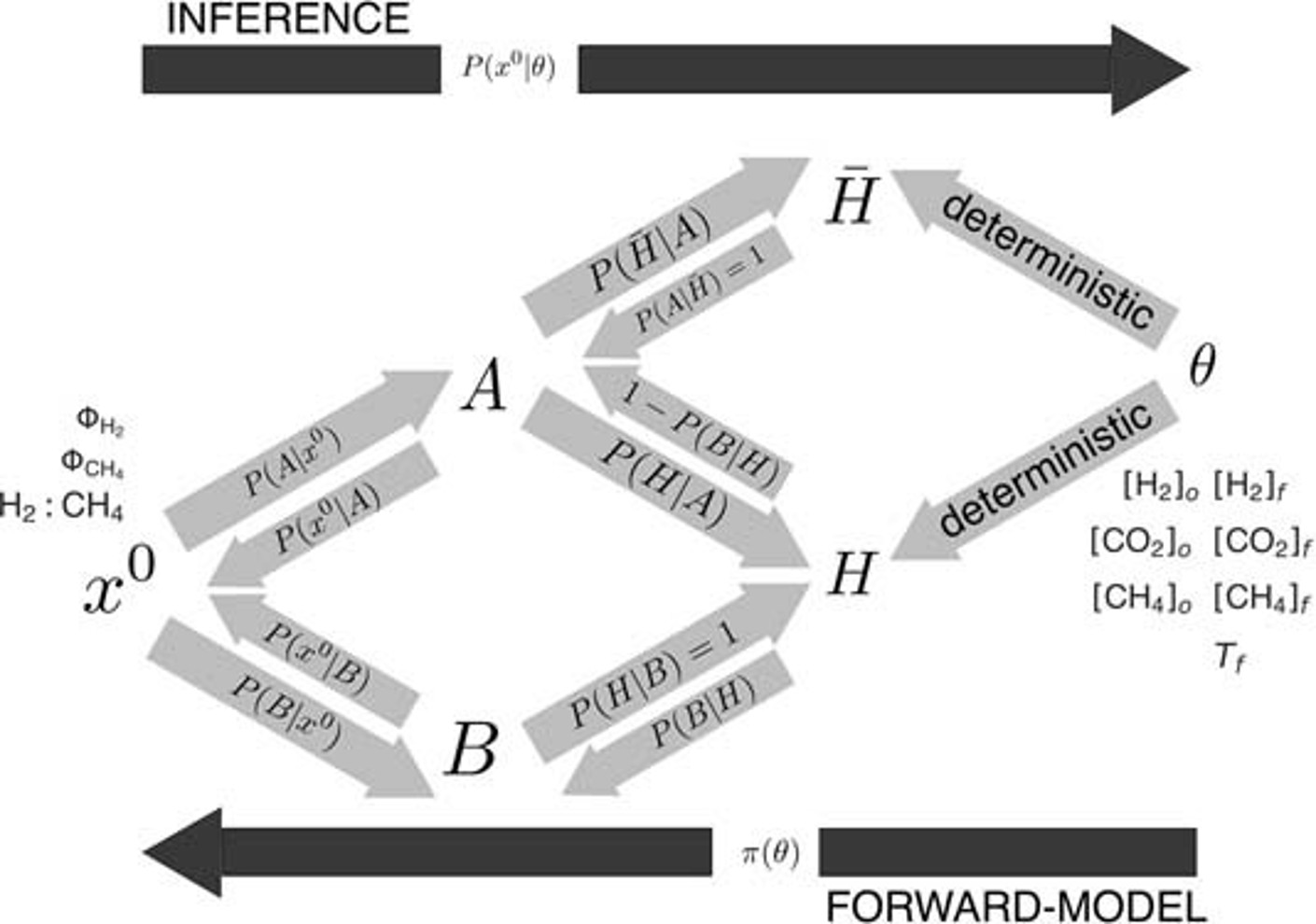
Fig. 5.62 Model framework for Enceladus’ ecosystem. At \(x^0\) are the observations, with \(\Phi\)H2 the flux of dihydrogen, \(\Phi\)CH4 the flux of methane, and the ratio H2:CH4 Theta are the model parameters which include the composition of Enceladus’ putative hydrothermal fluid and ocean as well as hydrothermal fluid temperature. The H denotes the habitability, and H bar, not habitable. X are the generated data, so \(x=\pi(\Theta)\) where \(\pi\) denotes a model. B is where the seawater composition is contributed to by biological processes and A is where its abiotic processes. From Affholder et al., (2021)#
In order to test the likelihood that the high H2 levels are biotically generated, Affholder et al. (2021) built an ecological model using Approximate Bayesian Computation (ABC) method to assess the likelihood of abiotic, habitable, habitable but uninhabited. In terms of the model set up (see Figure), there is H2 in the hydrothermal fluid and in the ocean. Dissolved inorganic carbon (DIC) is present in the fluid and in the ocean, methane in the fluid due to serpentinization only, in the hydrothermal fluid, and in the oceans. The aim is to work out \(P(B∣x^0)\) the probability of B, i.e. biotic activity given the observed parameters \(x^0\). This work was done by generating 50,000 simulations using random values of internal parameters drawn from the prior distributions of H2, DIC and CH4.
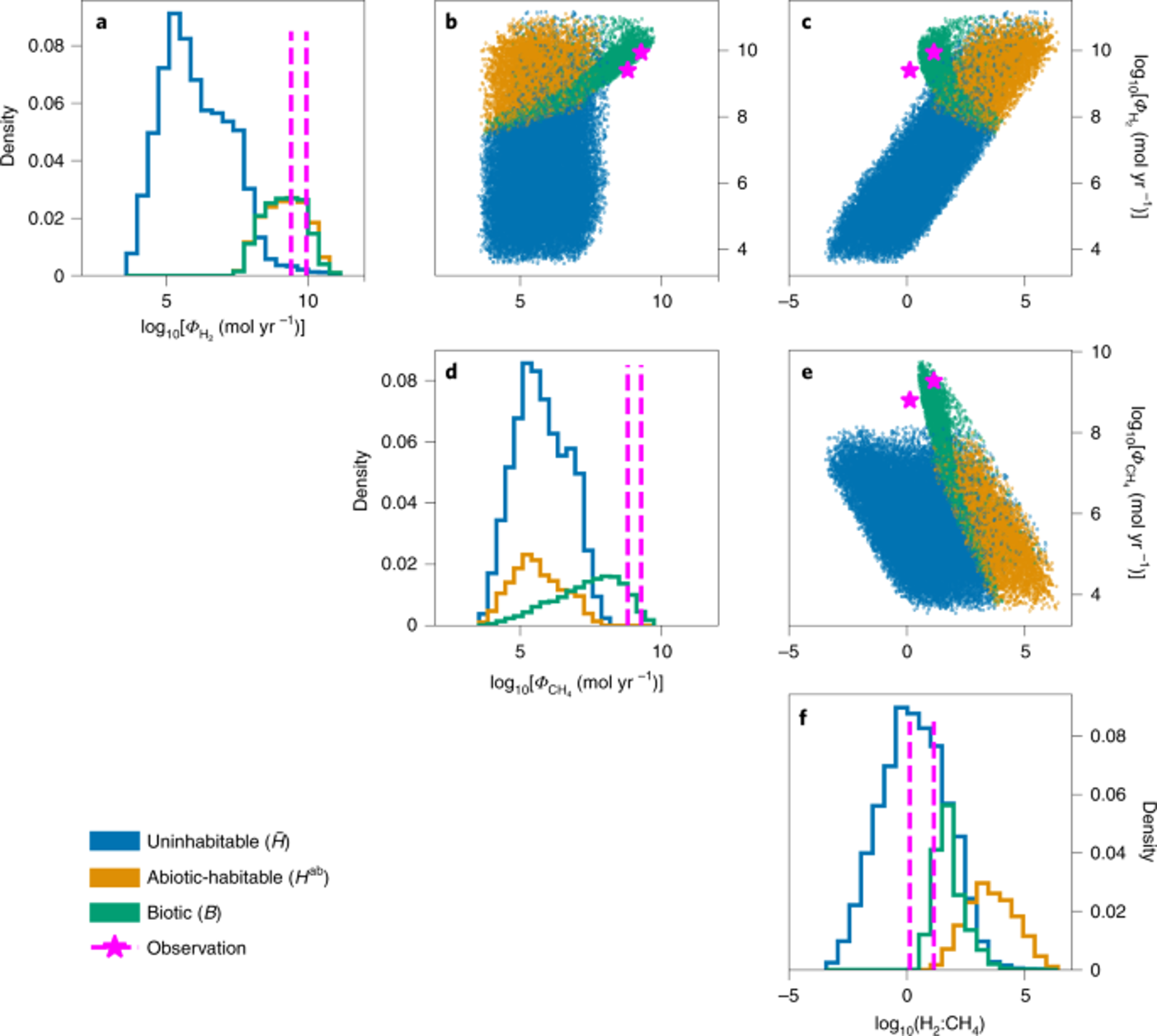
Fig. 5.63 The simulated model data for the H2 and CH4 fluxes (\(\Phi\)H2 and \(\Phi\)CH4; a and d, respectively) and for the H2:CH4 gas ratio. These fluxes and ratios are shown along the x axis on a log scale. The y axis are the posterior distributions. The blue shows the simulations whereby methanogens could not grow, orange is where methanogens could survive, don’t. The actual simulation results are shown in the dot plots, where we can see this blue cloud showing uninhabitable, orange habitable but abiotic, biotic in green, and observations in pink. B shows , \(\Phi\)CH4 versus \(\Phi\)H2. c, shows the H2:CH4 gas ratio versus \(\Phi\)H2. and e, shows H2:CH4 gas ratio versus \(\Phi\)CH4. Magenta stars indicate the Cassini observations. For b-e, there is a log scale on both axes. From Affholder et al., (2021)#
Fig. 5.63 shows how 68% the simulated results would not support methanogenesis. But for 32% of these simulations’ methanogens were possible, and the possible space overlaps with the observations.
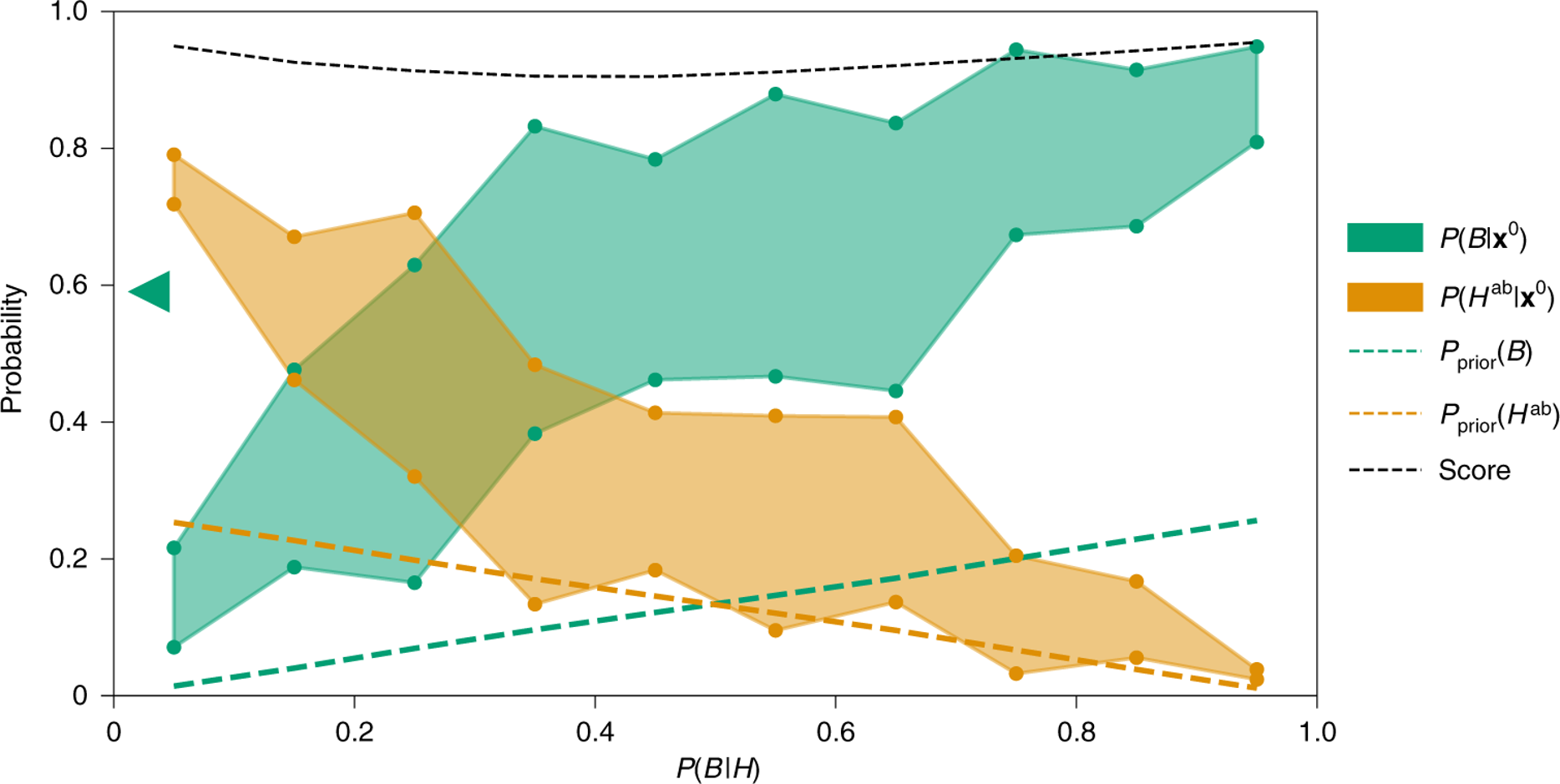
Fig. 5.64 The x axis is the probability of life emerging given a habitable environment, \(P(B∣H)\). For each \(P(B∣H)\) value, the circles (green or orange) indicate the posterior probability of the biotic scenario (B, green) and abiotic-habitable scenario (Hab, orange) for the lower and upper bounds of the observation range. The green triangle on the y axis shows the mean value of the posterior probability of the observations given biotic across the parameter ranges \(P(B∣x^0)\) which is 0.59 with the prior that all values of \(P(B∣H)\) are equally likely. The probability of the observations given unhabitability is very low, always less than both biotic of abiotic-habitable so isn’t shown. The green and orange dashed lines are the priors, and the black line is the RF-ABC classifier score. From Affholder et al., (2021)#
Only the biotic models have a non-zero likelihood for every observable (provided the change of life emerging is over 0.40). If \(P(B∣H)\) is less than 0.2, then we can see here that the preferred model is abiotic-habitable, between 0.2 and 0.4 they are equally likely, and above 0.4 then methanogenesis is the preferred model. Taken together this work shows that for the observed plume observations, they (1) can’t be explained just serpentinization, that is the abiotic reactions of the water with the rocky (2) they are compatible with habitable conditions for methanogens; and (3) if the chance of biotic given a habitable environment is above 0.4, then methanogenesis is the most likely case.
Biological evolution on different planets and moons?#
Modelling evolution on exoplanets is severely hampered by our lack of understanding to what drives the major evolutionary transitions. One conservative approach is to use neutral molecular evolution models to model speciation rates and evolutionary patterns: In the absence of any selection pressures, what would the macroevolutionary patterns be like? While we know these models can’t capture all the nuances of selection, because they can capture broad patterns, they can provide still novel insights into the overarching patterns. This approach starts with the metabolic theory of ecology whereby the metabolism of organisms from cyanobacteria to large fish can be predicted by environmental temperature and biomass. Since metabolism is strongly correlated with life history traits, and also evolutionary rates it means from just temperature and biomass it is possible to make predictions about evolutionary rates. Evolutionary rate is inversely proportion to the time to speciation, so linked to how long it would take to get origination of different organism groups (or clades).
This work focused on Hycean exoplanets which are class of habitable sub-Neptunes with diameters of ∼1–2.6 diameters of the sun with planet-wide oceans and H2-rich atmospheres which transit M dwarfs. They are particularly interesting to study in the context of life elsewhere in the universe because the volatile rich interiors lead to larger sizes and larger atmospheres compared to similarly sized rocky planets, making them more conductive to atmospheric observations.
For this model there are some simple assumptions. The first is that Life’s evolutionary transitions proceed deterministically as they have done on Earth. Secondly, life isn’t resource or nutrient limited. Thirdly, in this model, life can’t change the planetary temperature. This study focused on unicellular organisms to minimise assumptions made about the organisms. This metabolic theory of ecology can then be used to model how much evolution in terms of neutral nucleotide substitutions are needed for each clade. This value is then kept constant, with the temperature changed, and the time to origination of these groups output. The origination times of different key groups were then calculated for planetary temperatures of plus and minus 10 kelvin compared to Earth’s median temperature (this keeps the planet within the normal thermal ranges of most organisms (0-40\(^\circ\))). With just 10 degrees colder, only archaea will have evolved after 4 billion years, whereas at 10 degrees hotter, by 1.3 billion years post origination of life, all these major groups would have originated. This is important for detection, because more complex groups are more capable of producing stronger biosignatures.

Fig. 5.65 Time-calibrated phylogenetic trees with calculated evolutionary rates at Earth’s median temperature (top) and at +10 K increase relative to Earth (bottom) with the colour indicating the evolutionary rates at the nodes.#
Prospects for using astrobiology to understand evolution on Earth#
Part of the difficultly for understanding major transitions, such as the evolution of Eukaryotes or animals is that currently we only have n=1 for life. But there is the possibility that if we find life outside our own planet, because we go beyond this n=1, we have the potential to shed light on how likely these different transitions are. By comparing populations of biosignatures coupled to an understanding of what sort of biosphere they likely correspond to, we can compared them to what we would expect if life was deterministic and identical to Earth or if/how it was different. There is the potential to use the differences in timing and relative proportions of biosphere complexity to start to constrain the likelihood of each of these transitions and the conditions for them. So this information can be used to help understand whether life here on Earth is normal, and predictable, whether evolution is actually more variable, and different on other planets, and indeed what the likelihood of these different transitions actually is.