3.10. Mars III: Geophysics#
Professor: Nick Rawlinson (Department of Earth Sciences)
Key Concepts:
The geology and internal structure of Mars was not well understood prior to space missions, such as Mariner IV, which was the first flyby mission of the 1960s.
With subsequent space missions that achieved orbit, landings and rover deployments, geophysical datasets that provided detailed information on topography, gravity and magnetic fields, marsquakes, surface pressure etc. became available to the scientific community.
Although the Viking missions did record a few marsquakes, it wasn’t until the InSight mission in 2018 that high quality seismic recordings became available.
With just one seismometer located on Mars, the detection and location of marsquakes is a challenge. However, with clear identification of body wave phases and polarization analysis, approximate location is possible.
Most marsquakes were recorded from Cerberus Fossae, which was found to be an actively extending graben structure that is evidence of recent tectonics and magmatic processes in the lithosphere.
The Martian core is liquid and appears to be surrounded by a thin (~150 km thick) silicate layer that is also in a liquid state.
In this lecture, we will explore how geophysical observations of Mars have allowed us to illuminate its interior structure and processes, and provide fresh insight into the formation and evolution of terrestrial planets. Such observations come largely from space missions to Mars, which enable orbital or surface analysis of the planet. A rough timeline of the key missions will be presented below. How these observations have been used to understand the atmosphere, surface and interior of Mars will also be briefly discussed. In recent years, a significant step forwards in understanding the internal structure and dynamics of Mars was achieved through new seismic recordings from the InSight mission. Details of this mission and the earthquakes that were recorded will be presented, along with an example of how they can be used to infer the internal structure of the planet
A history of geophysical exploration on Mars#
After the Earth and Moon, Mars is the most explored planetary body in our solar system - not just because of its proximity, but also because of its tantalising similarity to Earth. Prior to space missions to Mars, its internal structure was poorly understood, with many workers concluding that it was undifferentiated and nearly homogeneous based on moment of intertia arguments (see Fig. 3.67)
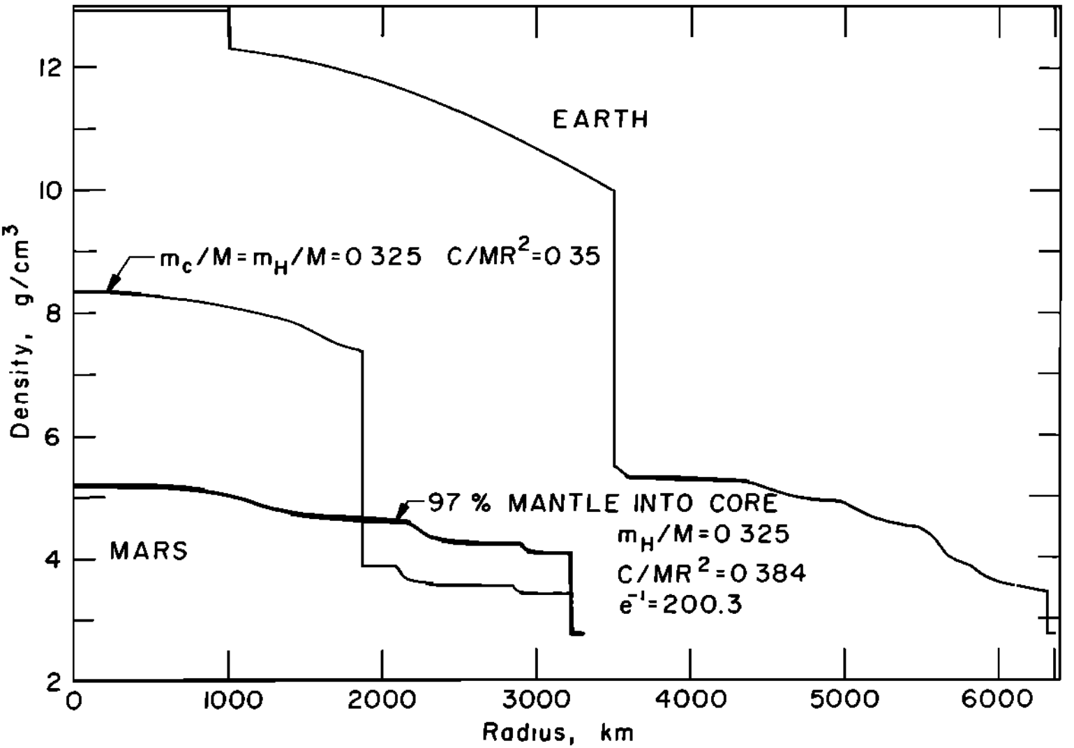
Fig. 3.67 Density structure of the Earth and Mars according to Kovach and Anderson (1965). The thick black line shows the preferred model, with the differentiated model “having too low a moment of inertia”.#
The first successful mission to Mars was achieved by NASA with Mariner IV in mid 1965. This was a flyby mission, in which the probe passed within 10,000 km of the Martian surface. Its main contribution to science came from photos of the surface of the planet (which showed a cratered and apparently lifeless surface), but it also measured daytime temperatures and surface pressure (in the latter case, by refracting radio signals through the Martian atmosphere - a process referred to as radio occultation), which was found to be very low (6-10 millibars). Mariner IV also carried two devices designed for detecting the magnetic field of Mars. However, from distances <13,000 km from the surface of the planet, no magnetic signature was detected by either instrument, a result which contrasted with that of the Earth.
Mariner VI and VII followed in 1969, and found that the atmosphere of Mars was made almost entirely of carbon dioxide (98%) and had surface temperatures ranging from -73 to -125 C. An ice cap was found to exist at the south pole, which was determined to consist largely of carbon dioxide. Radio occultation provided a means to accurately measure the mass, radius and shape of Mars, which ultimately helped to refute earlier claims that the planet is undifferentiated. An interesting fact is that the total data return from Mariner VI and VII combined was only 100 Mb.
The dawn of space missions to Mars also coincided with the depths of the cold war between the then Soviet Union and the United States of America. This was partly played out in space, with competing missions to the moon and Mars. In 1971, after s string of previous failures, the Soviet Union successfully launched Mars 2 and Mars 3, both of which were designed to go into orbit around Mars, send a lander to the surface, and deploy a rover. Both achieved orbit, but only Mars 3 managed a soft touchdown, after which it soon lost transmission, so the rover remained undeployed. Mars 2 successfully completed 362 orbits and sent back a large volume of data on atmospheric composition and surface temperatures. These missions were also notable for enabling the generation of surface relief maps and providing more details on gravity and magnetic fields.
Following Mars 2 and 3, a series of successful space missions that achieved orbits followed, both by the Soviet Union and United States. However, it wasn’t until Viking 1 in 1976 that a successful landing took place that was able to return useful data (Fig. 3.68). Viking 1 was able to take soil samples using a robotic arm, and take photographs of the Martian surface from close range. Viking 2 landed shortly afterwards, and was notable for its recording of Martian seismicity (Viking 1 also carried a seismometer, but it failed). However, due to wind and lander noise, it was only able to record two marsquakes.
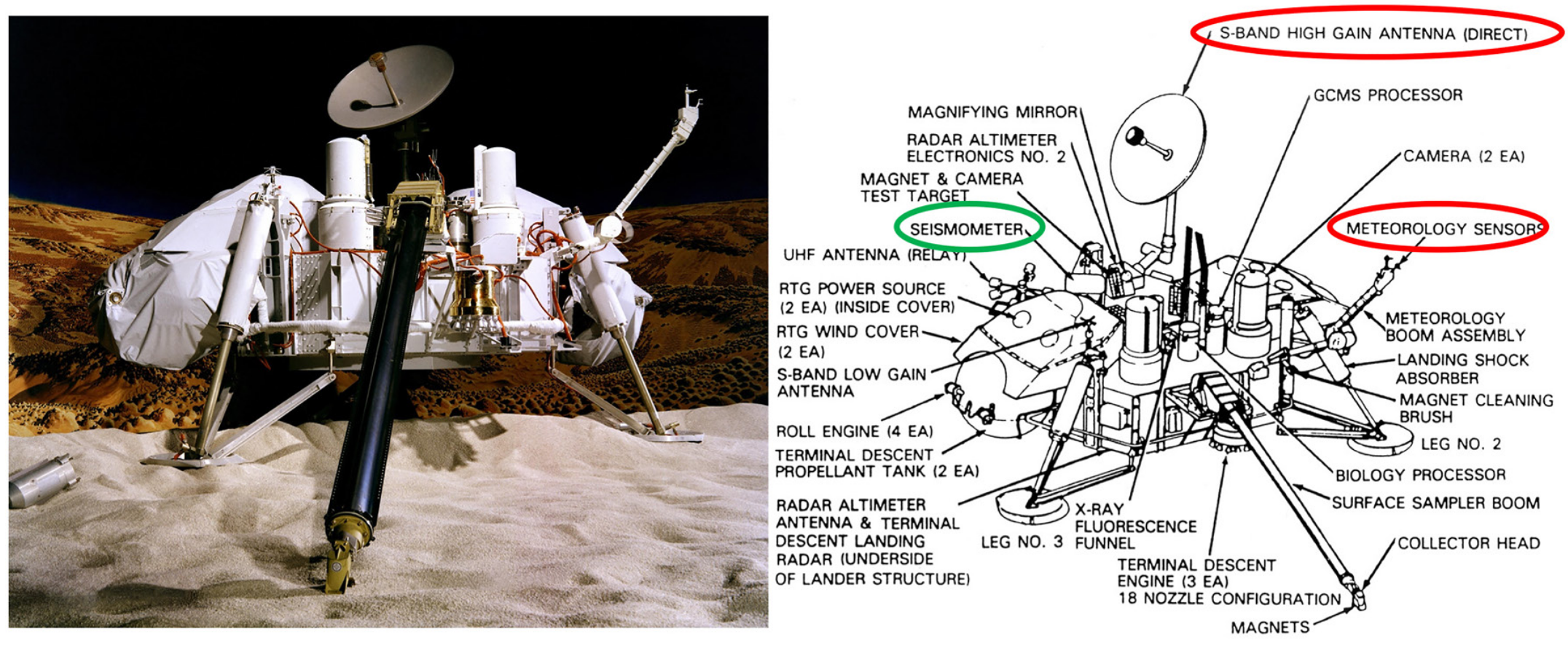
Fig. 3.68 Design of the Viking lander. Note that the seismometer is mounted on the lander, which resulted in high noise levels due to exposure to wind and lander noise (Lazarewicz, 2023).#
Following the successful Viking Missions, there was somewhat of a hiatus in Mars missions, partly due to launch and other failures, but from the 1990s onwards, missions became more regular. Those that are more notable in terms of geophysics include the Mars Global Surveyor, which carried a laser altimeter, magnetometer and device for measuring the gravitational field. These precise measurements allowed for inferences to be made about the crust and upper mantle structure beneath the martian surface (Zuber et al., 2020). The Mars pathfinder mission that achieved a landing in 1997 was the first mission to successfully deploy a rover. However, from a geophysical point of view, it was the accurate measurements of the planet’s moment of inertia which lead to a rethink of planetary accretion models. A number of missions followed that included landings on Mars, including Spirit, Opportunity, Phoenix and the Mars Science laboratory. However, these were largely focused on the search for water and evidence of life. The Insight mission, which landed on the surface of Mars in November 2018, was the first mission with a geophysics focus, and will be discussed in more detail below.
Seismology on Mars#
The Insight mission represents a geophysical step-change for Mars, since it successfully deployed a 3-component broadband seismometer on the planetary surface. This instrument, called SEIS (Seismic Experiment for Interior Structure), comprises a 3-axis very broadband seismometer beneath a heavy wind and thermal shield, designed to minimise the noise caused by wind and temperature variations. The peak sample rate used was 100 sps, which limited maximum frequencies to 50 Hz.
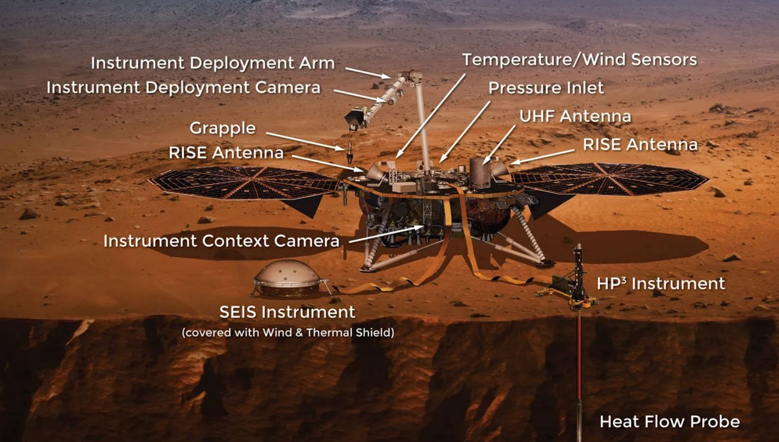
Fig. 3.69 Design of the InSight lander, showing the seismometer on the surface following its deployment by a robotic arm (from Nasa).#
SEIS recorded for a period of just over four years, during which time it detected 1319 marsquakes. This compares to 35,000 moonquakes detected during the Apollo missions from 1969-1977; in fact, this large number of moonquakes gave rise to the expectation that more marsquakes would be discovered by InSight. Marsquakes are characterised by their dominant frequency content, from high frequency (>2.4 Hz), broadband (low frequency up to 2.4 Hz) and low frequency (below 1 Hz). Event detection was found to be heavily dependent on the ambient noise conditions at the lander, with Martian autumn and winter proving particularly noisy. Fig. 3.70 clearly shows that noise levels are too high during the Martian day to permit detection except for large or nearby events; similarly, noise conditions during winter months, even during the night, are such they they largely preclude detection,
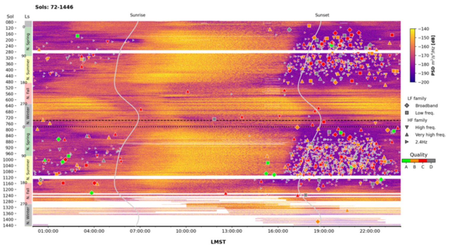
Fig. 3.70 Daily spectogram of the very broadband vertical component of SEIS from sol 72 to 1446, noting that one sol is approximately 40 minutes longer than a day on Earth. Catalogued seismic events are superimposed (from Horleston, 2023).#
The detection and location problem#
With just one seismometer, the detection problem becomes harder, but the location problem may at first seem impossible, unless there was complementary evidence e.g. space-based detection of an impact. On Earth, large national and global networks are routinely used for detecting and locating earthquakes, and it is well recognised that at least three seismometers are needed to achieve a well-constrained location, with noise and other factors including seismic model accuracy contributing to location uncertainty. If an arrival consisted of a single impulse on all components, then indeed location would be out of the question. But seismic waves are elastic waves that exhibit particle motion in all direction, and whether on Mars or Earth, they travel through a heterogeneous structure that adds to their complexity.
Fig. 3.71 shows a distant earthquake recorded by a single 3-component broadband seismometer on Earth. It is easy to see that it contains a huge amount of information. P-waves and S-waves are compressional and transverse waves, respectively, which travel through the body of the Earth, They can reflect, refract and mode convert at a boundary according to Snell’s law to produce multiple paths. If there is a reasonably accurate model of P-wave and S-wave speed for Mars, then it is relatively straightforward to match these phase arrival times to model predictions, which would yield a constraint on epicentral distance. It turns out that such models were available even before InSight landed on Mars, and although seismic recordings enabled improvement, they were a reasonable approximation (based on radial estimates of density, composition and pressure). In terms of backazimuth location (orientation from the receiver to the earthquake), this can be estimated from the polarization of arriving seismic energy. A clear example in Fig. 3.71 is shown by the surface waves, with Rayleigh waves appearing on the radial component (direction between the source and receiver) and vertical component, while faster-arriving Love waves appear on the transverse component (direction perpendicular to the radial component in the horizontal plane).
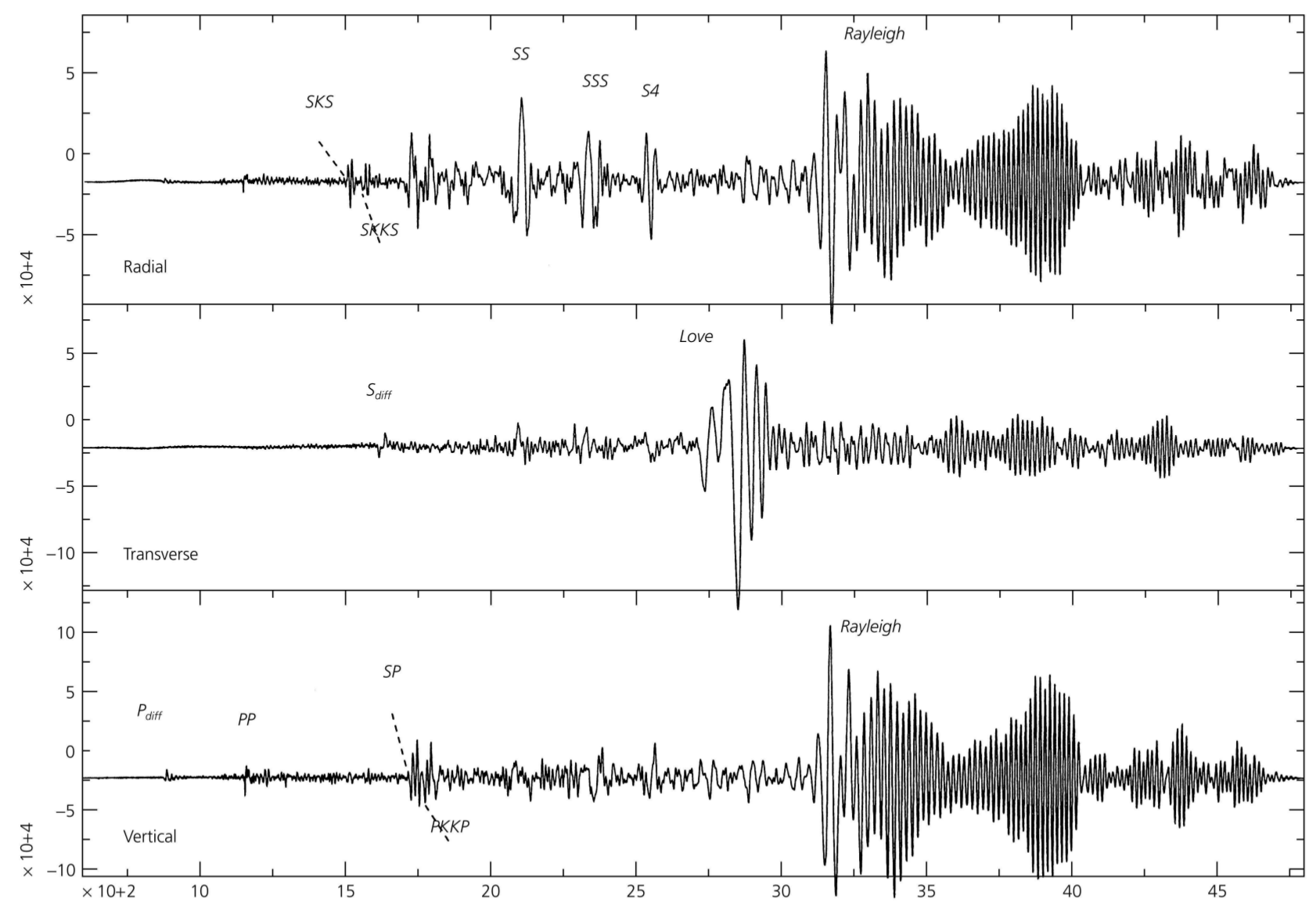
Fig. 3.71 A three-component broadband seismogram from a distant Earthquake recorded on Earth. The body wave portion (lower amplitude first arriving wavetrains) of the seismogram contains many distinct arrivals. Large amplitude surface waves can be seen to trail the body waves (from Stein and Wysession, 2003).#
As such, the complete location problem is potentialy solvable given a 3-component seismogram recorded at a single location; the main limitation will be on accuracy. If later arriving body wave phases, such as pP are available, control of depth can actually be quite good; however, if these so-called depth-sensitive phases are not present, then depth constraints will likely be poor. Fig. 3.72 shows a range of body wave path signatures for the Earth, and the accompanying move-out curves, which illustrate how their arrival time varies with epicentral distance. It is easy to see from this that provided several body wave phases are present in a seismogram, determining an approximate epicentral distance is not difficult.
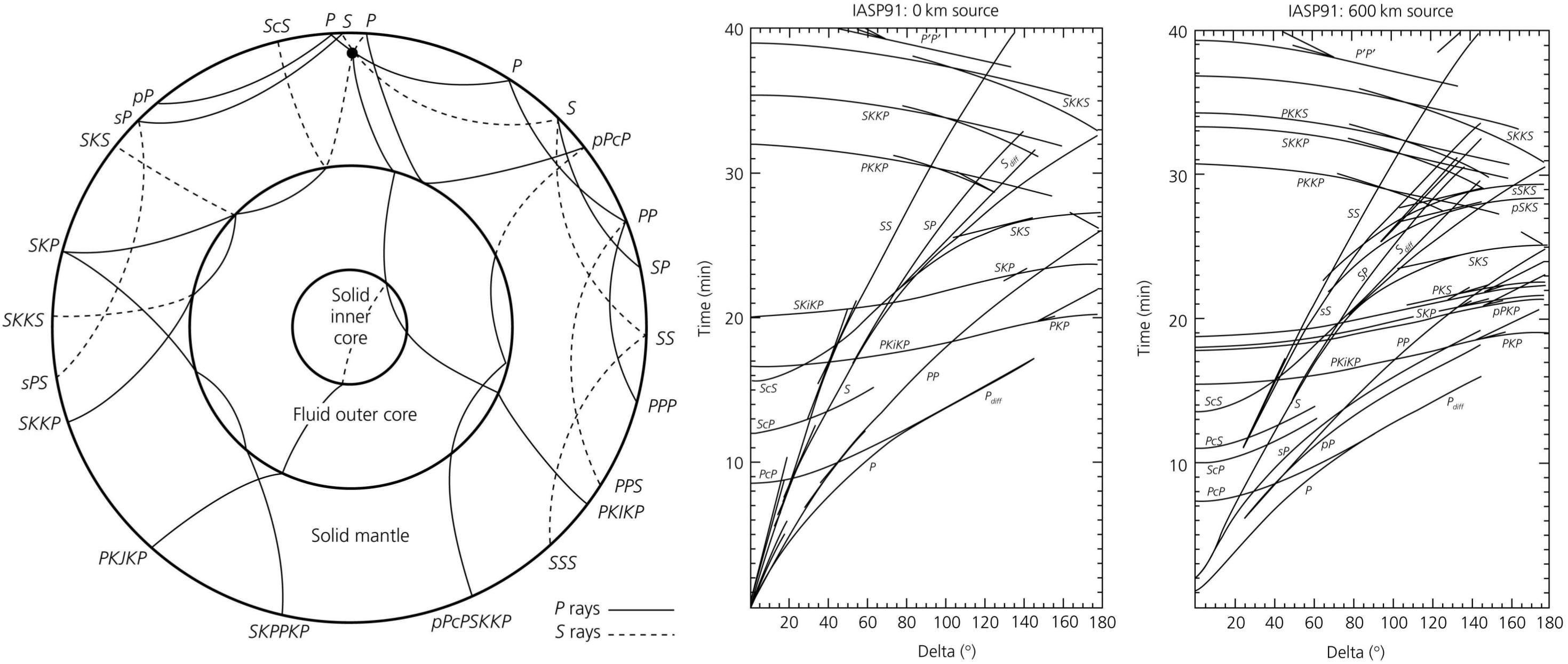
Fig. 3.72 Left: Path signatures of various body wave phases in the Earth. Middle: Corresponding traveltime curves for a source at the surface; Right: Corresponding traveltime curves for a source at 600 km depth. (from Stein and Wysession, 2003).#
While surface wave polarization can be used to determine source backazimuth, body wave polarization methods tend to be used in practice (Frohlich and Pulliam, 1999), for example using the polarization of the P-wave arrival and its coda, which often are easiest to identify on a seismogram and are not contaminated by other phases. Similar methods tended to be used with InSight data - for example, Drilleau et al. 2022 computed backazimuth under the assumption that in this direction, the expectation is that energy is maximum, and the correlation coefficient and instantaneous phase between vertical and horiztonal components is negative and minimum.
Apart from having to rely on data from just a single seismometer, another challenge for earthquake location on Mars is the intense scattering observed in marsquakes records. This results in the smoothing of impulsive arrivals and the generation of long coda, which reduces the number of clear P- and S-wave arrivals.
InSight was also able to detect meteoroid airbursts and impacts, despite initial expectations that it may be challenging, with prelaunch estimates ranging from 1-10/year for impacts and 10-200/year for airbursts. In the first year, no impacts were detected, whereas in the second year, 6 impacts were detected. Fig. 3.73 shows a map of Mars seismicity, as detected by InSight. The significant uncertainty in location (given by the black lines) is to be expected, given that data from only a single seismometer is used.
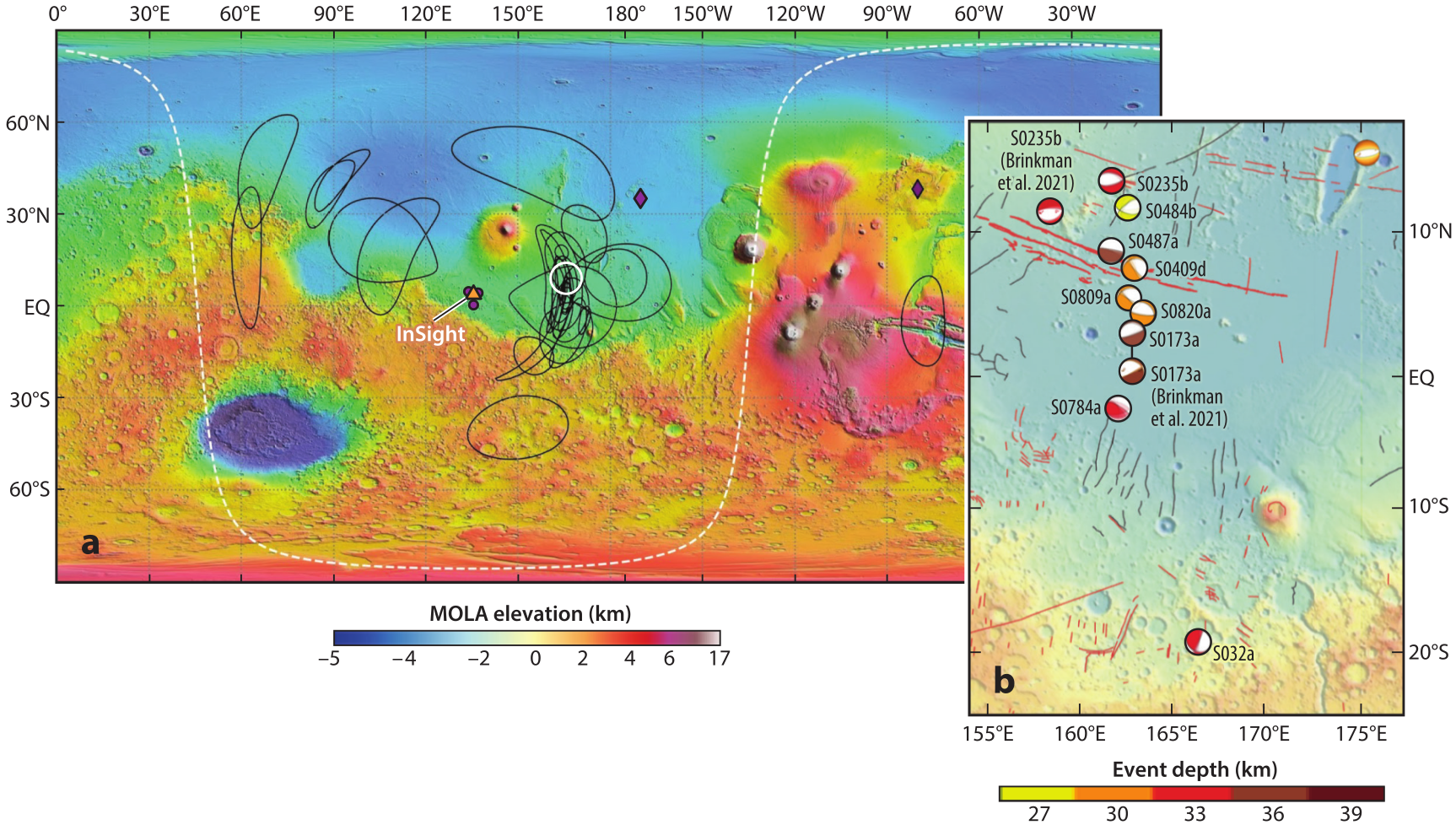
Fig. 3.73 Location of Marsquakes as determined from data collected by the InSight mission. The orange triangle indicates the location of the lander. Black ellipses indicate location uncertainty associated with the low frequency family of events. Purple symbols indicate locations of events that were determined to be impacts (diamonds are large impacts, while circles are small impacts close to the lander). The white circle denotes the location of a cluster of high frequency events. The dashed white line indicates an angular distance of 90 degrees from the lander. Inset: CMT focal mechanisms for events in the neighbourhood of Cerberus Fossae (from Lognonne et al., 2023).#
The distribution of marsquakes during the operational period of SEIS is irregular, but one consideration is that smaller events are more easily detected close to the lander, as implied by Fig. 3.74, which shows the complete set of marsquakes plotted as a function of epicentral distance from the lander and moment magnitude.
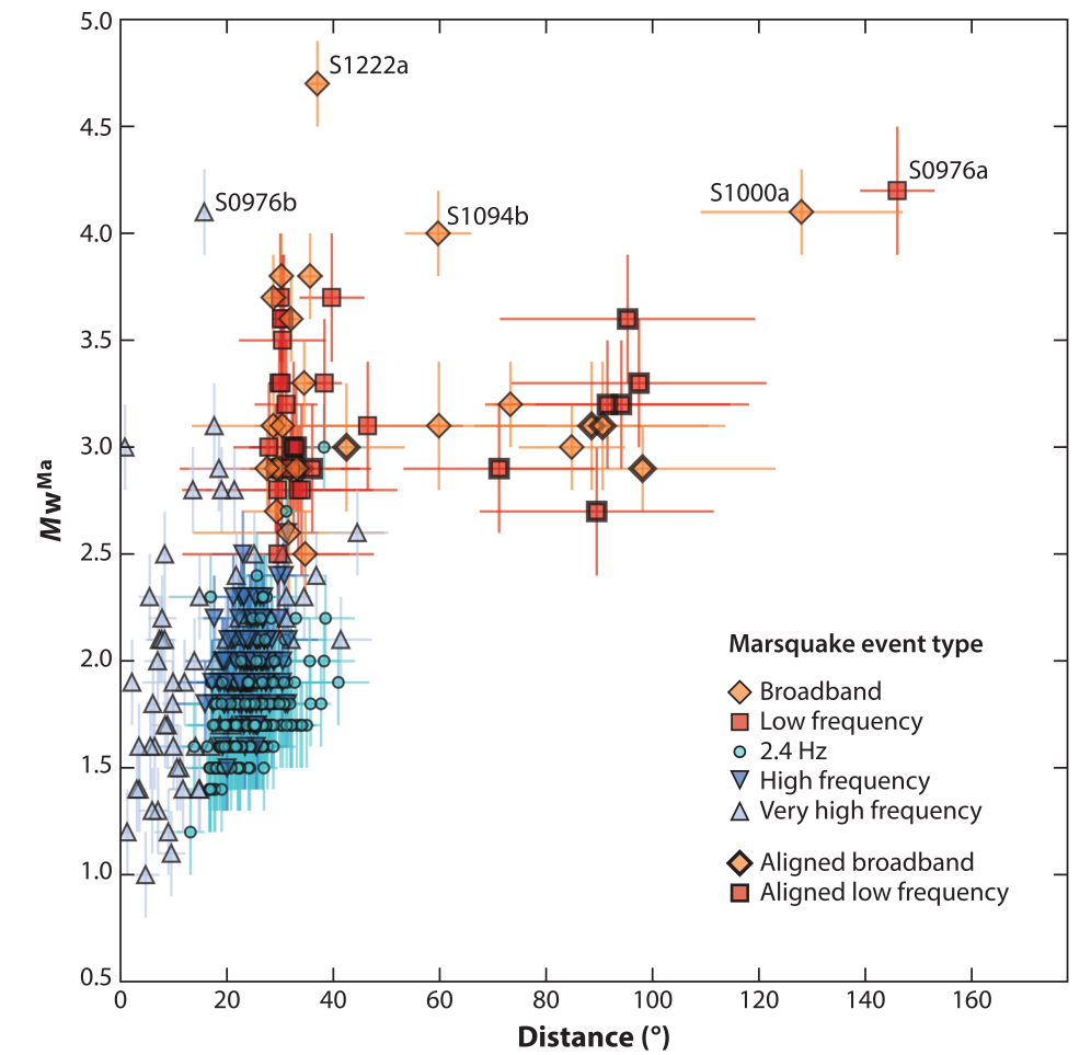
Fig. 3.74 Marsquakes plotted in terms of moment magnitude as a function of epicentral distance from the lander. Two of the larger events, S1000a and S1094b are impacts. Note the size of the uncertainty in both epicentral distance and moment magnitude (from Lognonne et al., 2023).#
Cerberus Fossae#
The largest concentration of marsquakes occurs in the nieghbourhood of Cerberus Fossae, and is likely a reflection of ongoing tectonic activity. It lies approximately 1,200-2,300 km east of the lander, and appears to be a dyke-induced graben system, or a system of collapsed and widened volcanic fissures, which produces an elongated depression. Active volcanism in the region is thought to have ended less than 10 Ma. Based on ths distribution of seismicity, their frequency content and moment release, Stahler et al., 2022 conclude that Cerberus Fossae is still actively opening under the influence of an extensional stress regime located in a warm source region beneath. They propose that shallow seismicity from high frequency events is created by ruptures at shallow depth due to the graben structure itself (see Fig. 3.75). More broadly, they conclude that lithospheric compression is not the dominant driver of contemporary tectonics on Mars.
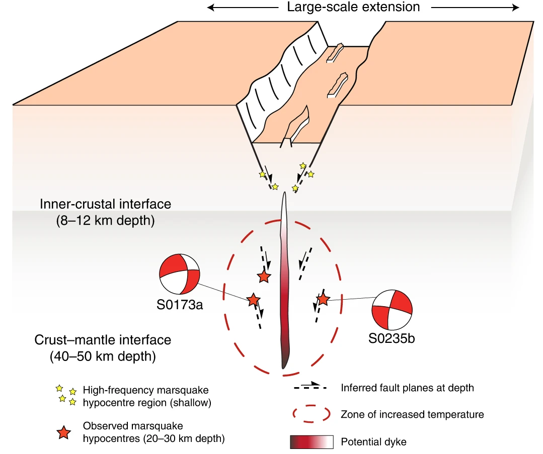
Fig. 3.75 Relationship between active opening of Cerberus Fossae and seismicity recorded by InSight (From Stahler et al., 2022).#
The Martian core#
Largely using marsquake seismicity recorded by InSight, there has been a whole raft of papers that have studied the structure of the Martian interior from crust to core. The radius and composition of the core has been a key topic, particularly in light of the difficulties in determining these parameters prior to InSight. In a recent study, Khan et al. 2023 used core-sensitive body waves generated by low frequency marsquakes and meteor impacts to make inferences about the state and composition of the Martian core. They found that the best fit to the data and prior information of the thermoelastic properties of liquid iron-rich alloys require that a fully molten silicate layer, about 150 km thick, wraps itself around a smaller, denser liquid core of radius 1,675 km. The core is determined to contain 85—91 wt% iron-nickel and 9—15 wt% light elements, primarily sulfur, carbon, oxygen and hydrogen. Fig. 3.76 provides a summary of these results, including the path signatures used to help determine the presence of a molten silicate layer.
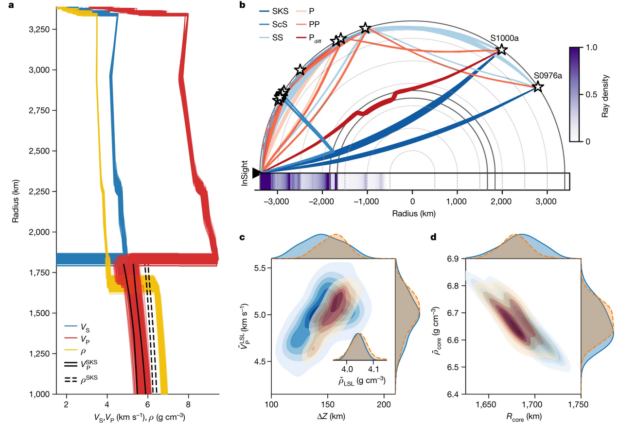
Fig. 3.76 a: P-wave, S-wave and density profiles obtained from inversion. For comparison, black solid and dashed lines represent the range of core profiles determined previously using SKS phases. b: Body wave ray path geometry for all events used in the study. Colour bar denotes ray path density. c: Inverted molten silicate layer (LSL) properties. d: Inverted core properties. Blue and orange shaded distributions on top and to the right of c and d indicate sampled probability distributions for the various parameters shown in the plots (From Khan et al. 2023).#