2.5. The Evolution of Stars#
Professor: Christopher Tout (IoA)
Learning objectives:
The basic physics of stars illustrated by the structure equations.
The factors driving stellar evolution: nuclear burning and mixing, convection.
The respective evolutionary trajectories of low-, intermediate- and high-mass stars.
Outcomes of stellar death: supernovae, white dwarfs, neutron stars and black holes.
Stars appear to be of different brightness and colour. Knowing their distance we can place them in a Hertzsprung–Russell diagram that plots luminosity as a function of surface effective temperature. Stars then fall into distinct groups and evolve from one to another. We shall examine the physics that determines the structure of stars and thence their position in this diagram. There are two structure equations that describe conservation of mass and hydrostatic equilibrium. These are linked by an equation of state that relates pressure to temperature density and composition. To close the system two more equations are required for heat transport and energy generation. These equations determine the structure of a star. Stellar evolution is driven primarily by nuclear burning that changes the composition over time. Towards the end of a star’s life, mass loss in stellar winds becomes increasingly important. We shall discuss the evolution of a typical \(5\,M_\odot\) star.
The Hertzsprung–Russell Diagram#
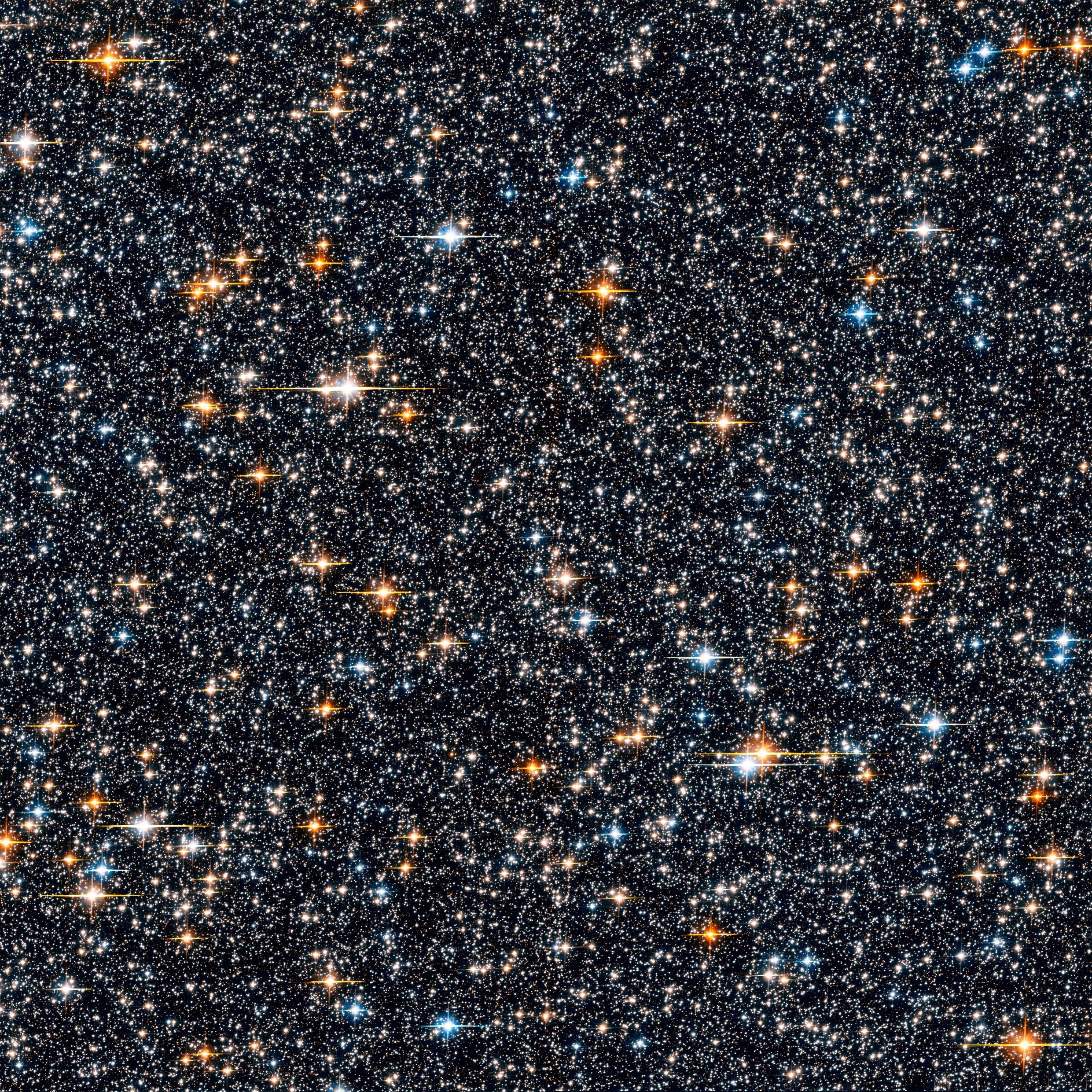
Fig. 2.27 Stars vary in brightness and colour#
Knowing the distance to a star we can measure its absolute luminosity \(L\). Stars are almost black bodies so define an effective temperature \(T_{\rm eff}\) such that
\(L = 4\pi\sigma R^2T_{\rm eff}^4.\)
Effective temperature can be determined from colour
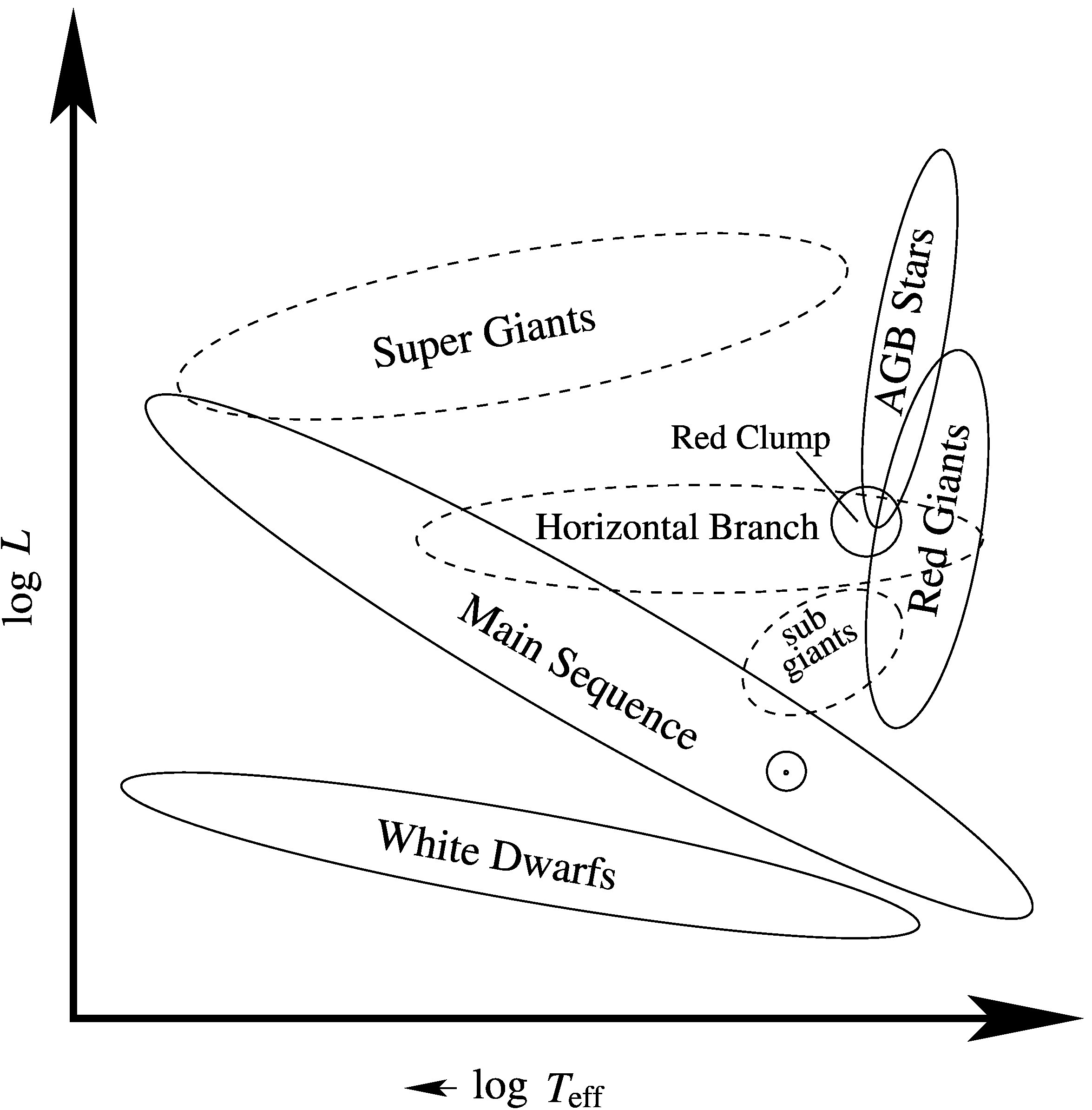
Fig. 2.28 A Hertzsprung–Russell Diagram showing various groups of stars that show up as distinct groups.#
stars that show up as distinct groups.
Now
\(\log L = 2\log R + 4\log T_{\rm eff} + \rm const\)
so loci of constant radius are straight lines in the H–R diagram with radius increasing towards the top right.
Stellar Types#
Main Sequence – the most populated region on which the Sun lies
Red Giants – a well populated area of large red stars
White Dwarfs – Faint small stars
AGB Stars – asymptotic giant branch stars, a more luminous sequence slightly offset from the red giants
subgiants – a sparsely populated group between the main sequence and giant branch
Super Giants – bright large stars spanning blue to red found in young star clusters
Red Clump – an increased population at the base of the AGB
Horizontal Branch – a similarly luminous set of stars extending bluewards from the red clump
Through steallr modelling we now have a good qualitative understanding of how stars evolve in an H–R diagram.
Structure Equations#
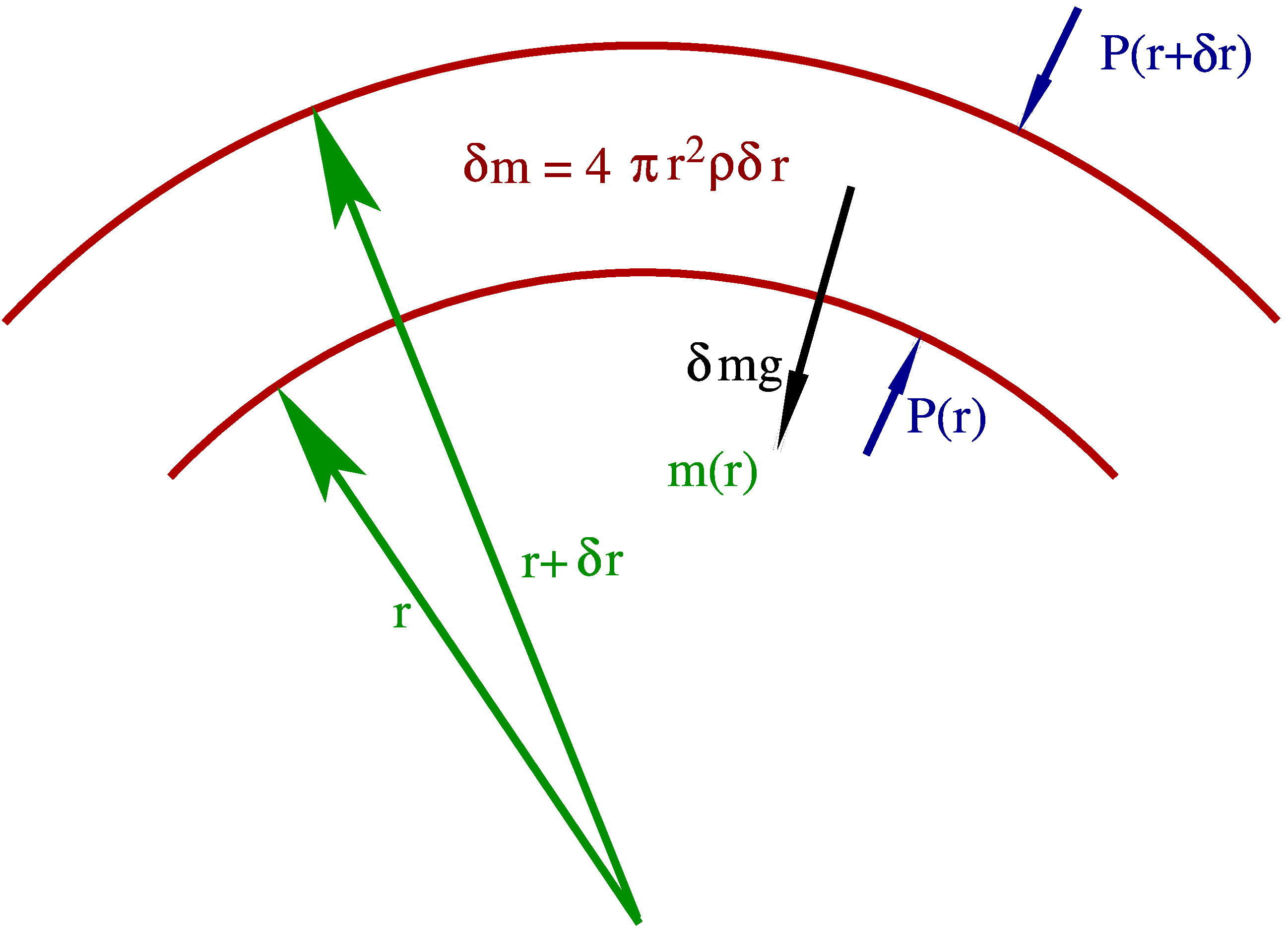
Fig. 2.29 Structure Eqautions.#
Conservation of mass
\({{\rm d}m\over{\rm d}r} = 4\pi r^2\rho\)
and hydrostatic equilibrium
\({{\rm d}P\over{\rm d}r} = -\rho g = -{Gm\rho\over r^2}.\)
Equation of state#
To relate pressure and density we must take into account temperature \(T\) and composition as well.
\(P = P_{\rm i} + P_{\rm e} + P_{\rm r}.\)
Ion pressure is typically perfect gas and can include electrons (gas pressure \(P_{\rm g} = P_{\rm i} + P_{\rm e}\)) at low enough density.
\(P_i = {\rho kT\over \mu m_{\rm H}},\)
where \(k\) is Boltzmann’s constant, \(m_{\rm H}\) is the mass of a hydrogen atom and \(\mu\) is the mean molecular weight. When electrons are included
\({1\over\mu}\approx 2X + {3\over 4}Y + {1\over 2}Z,\)
where \(X\) is the mass fraction of hydrogen, \(Y\) that of helium and \(Z\) that of everything else, often called metals. Changes in \(\mu\) drive evolution.
\(P_{\rm e}\) is electron degeneracy pressure, a quantum mechanical effect. The Heisenberg uncertainty principle, that we cannot know the position and velocity of a particle at the same time, means that as electrons are squeezed into smaller and smaller volumes the must move faster. This requires work and so exerts a pressure.
Radiation pressure
\(P_{\rm r} = {1\over 3}aT^4,\)
where \(a\) is the radiation constant, is important in hot regions of massive stars.
Energy Transport by Radiation#
Suppose a photon typically moves a distance \(\lambda\), its mean free path, between emission and absorption or scattering. Consider two surfaces in a star separated by \(\lambda\) with one slightly hotter, by \(\delta T\). Both emit energy as black bodies.
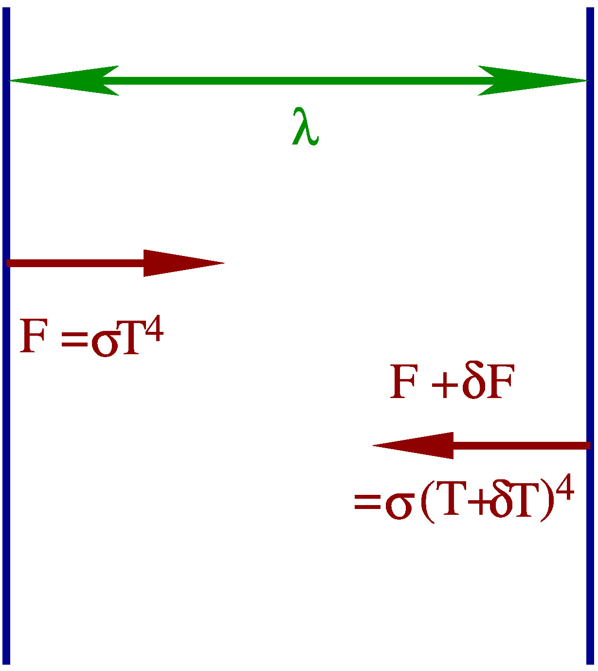
Fig. 2.30 Radiation transport.#
There is a net radiation flux \(\delta F\) from the hotter to the cooler surface. In a spherical star this amounts to a local luminosity
\(L_r = 4\pi r^2\delta F.\)
Now
\(\delta F \approx -4\sigma T^3\delta T\)
and we can relate \(\delta T\) to the temperature gradient
\(\delta T = \lambda{{\rm d}T\over{\rm d}r}.\)
We also relate \(\lambda\) to the opacity \(\kappa\), the cross-section per unit mass of stellar material so that
\(\rho\kappa\lambda = 1.\)
Combining everything and using \(\sigma = ac/4\), where \(c\) is the speed of light, we arrive at
\({{\rm d}T\over{\rm d}r} = {-\kappa\rho L_r\over 4\pi acr^2T^3}.\)
This is almost correct but we have negelected the fact that photons don’t necessarily travel directly between the surfaces and should also have integrated over all photon paths. Had we done so we would arrive at
\({{\rm d}T\over{\rm d}r} = {-3\kappa\rho L_r\over 16\pi acr^2T^3}.\)
Sources of opacity include electron scattering, absorption by electrons around ions, molecular absorption etc.
Convection#
When the temperature gradient is large energy can be transported by bulk motion of the fluid. Consider displacing an element of fluid upwards against gravity in the star.
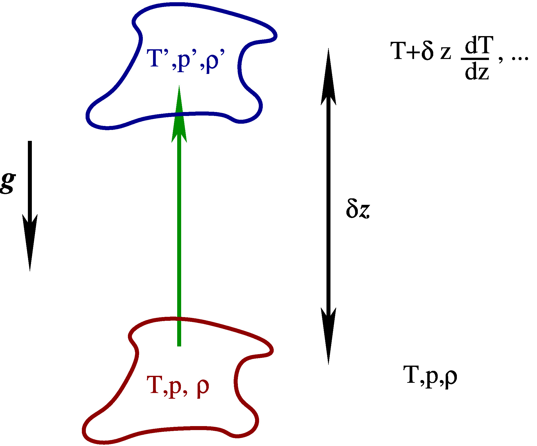
Fig. 2.31 Convection#
The element must remain in pressure equilibrium with its surroundings but does not immediately give up its heat. It behaves adiabatically and so its temperature and density adjust. If the element is then less dense than its surroundings it continues to rise carrying energy with it until it eventually disipates at some larger radius. Stellar material must be unstable to convection if its radiative temperature gradient
\(\nabla_{\rm rad} = {3\kappa PL_r\over 16\pi acGT^4m} > \nabla_{\rm ad} = \left({\partial\log T\over\partial\log P}\right)_S,\)
its adiabatic temperature gradient, at constant entropy \(S\). In general convection is very efficient so that convective zones in stars are isentropic with temperature gradient equal to adiabatic throughout. Importantly composition is mixed in convective zones.
Energy Generation#
Figure 5: Energy generation.
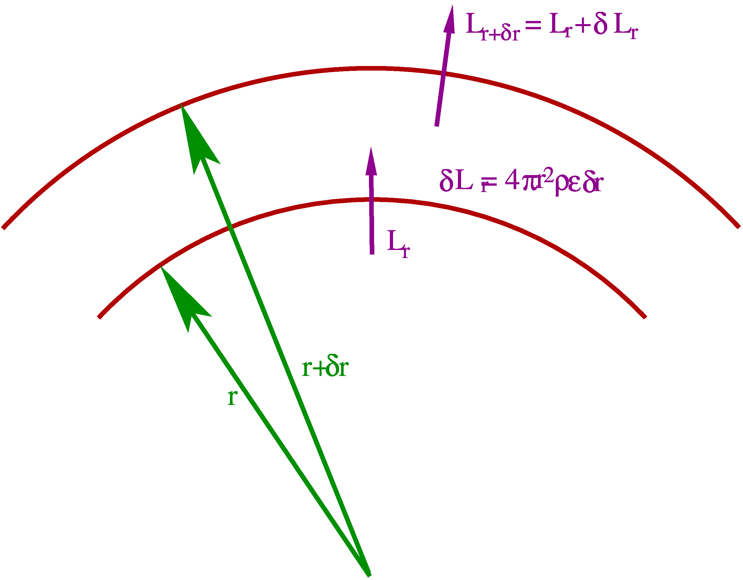
Fig. 2.32 Energy generation#
The stellar luminosity is generated at a rate \(\epsilon\) per unit mass. So
\({{\rm d}L_r\over{\rm d}r} = 4\pi r^2\rho\epsilon.\)
Nuclear reactions – the major source of energy in a star. The mass of a helium nucleus is slightly less than four protons plus two electrons so nuclear fusion creates energy from matter. For reactions to take place we require both the high end of the particle energy distribution and quantum mechanical tunelling. As a result reactions are very temperature sensitive and so tend to be thermostatically controlled, around \(2\times 10^7\,\)K for hydrogen burning and \(10^8\,\)K for helium burning.
Gravitational contraction – in the absence of nuclear reactions pressure support is lost and a star gradually contracts releasing gravitational energy. This is importnat during star formation.
Neutrino losses – some energy is always lost by neutrinos during fusion but at high denisities and temperatures neutrinos can be spontaneously produced. For instance very high energy photons can spontaneously create an electron and positron pair. Normally these anihilate to form another photon but rarely a neutrino and an antineutrino. Neutrinos have a tiny cross-section to stellar material and so escape from the star extracting energy.
The Main Sequence#
Approximately luminosity
\(L_{\rm MS} \propto M^3\)
while available fuel
\(E_{\rm tot} \propto M\)
so lifetime \(\tau_{\rm MS} \propto M^{-2}.\)
The remaining lifetime is about \(0.1\tau_{\rm MS}\). For the Sun \(\tau_{\rm MS}\) is about \(10\,\)Gyr.
Stellar Evolution#
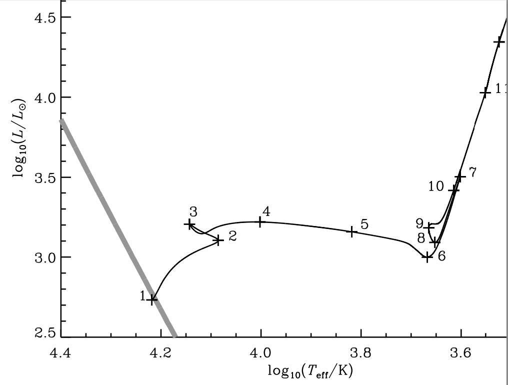
Fig. 2.33 The evolution of a \(5\,M_\odot\) star.#
1 – zero age main sequence, \(t = 0\), \(X = 0.7\) throughout, convective core burning
2 – \(X_{\rm c} = 0.029\), \(t = 100\,\)Myr star contracts a bit
3 – \(X_{\rm c} = 0\), shell burning begins
4 – \(M_{\rm c} = 0.63\) gas pressure can no longer support the isothermal core
5 – Hertzsprung gap, sub-giant phase, rapid evolution
6 – base of the giant branch, a deep convective envelope dredges into the old core
7 – core helium burning begins non-degenerately
8 to 10 – core helium burning, the red clump
10 – helium shell burning begins, the AGB
11 – second dredge up, burning shells become very close
12 – thermal pulses
13 – Degenerate carbon ignition, real stars lose their envelope before this to expose a carbon/oxygen white dwarf.
A \(1\,M_\odot\) star evolves similarly except that a) main-sequence hydrogen burning is radiative, b) helium ignites degenerately in a thermonuclear runaway, the helium flash, and c) there is no second dredge up.
Massive stars, above \(15\,M_\odot\) ignite helium in the Hertzsprung gap.
Stellar Remnants#
The final stages of a star’s life are a competition between nuclear burning and mass loss. Removal of a star’s envelope ends its life.
\(M < 0.9\,M_\odot\) – envelope lost on the RGB – He white dwarf \(0.9 < M/M_\odot < 8\) – on the AGB – CO white dwarf \(8 < M/M_\odot < 8.5\) – on the SAGB – ONeMg white dwarf
\(8.5 < M/M_\odot < 25\) – iron core reaches the Chandrasekhar mass – neutron star
\(M > 25\,M_\odot\) – envelope lost during core helium burning – naked helium star – neutron star or black hole
Evolution can be very different when a star has a close companion.