3.4. Planetary cycles I: Mantle Convection

Lecturer: David Al-Attar (Department of Earth Sciences)

---

Learning objectives:

• The Earth’s mantle exhibits a time-dependent rheology. Over time-scales of millions of years, it behaves like a viscous fluid.

• Viscosity is a strongly decreasing function of temperature. The cool outer part of the Earth is known as the lithosphere, and responds elastic over geological time. It is the warmer regions below the lithosphere that undergo convection.

• Scaling analysis to derive the Rayleigh number and understand its implications.

• The Earth’s mantle has a high Rayleigh number, and so must undergo vigorous time-dependent convection over a range of length-scales.

• Convection in the mantle contributes to long-wavelength gravity anomalies and dynamic topography at the Earth’s surface.

Introduction

The aim of this lecture is to summarise the key physical principles governing convection within the Earth’s mantle. Though our focus is on the Earth, the same rules, presumably, apply within other Earth-like planets.

Mantle rheology

Mantle convection can be understood in terms of fluid mechanics. But the Earth’s mantle is very much a solid. This apparent contradiction is resolved by the mantle’s time-dependent rheology: over short timescales (like for seismic waves) it is a solid, but over geological timescales, it flows like a very viscous fluid. To understand this, we need to consider the rheological behaviour of the mantle. By the rheology of a material we mean the quantitative relationship between deformation and stress. The key idea is that the mantle exhibits a time-dependent rheology, this meaning, roughly, that the response to forcing depends on the time-scale over which it is applied.

Within the following discussion we will write \(\sigma\) for the stress and \(\epsilon\) for the strain. Strictly, these are tensor-fields, but this is not important for the moment.

End member behaviour

To begin, we consider two simple rheologies that describe the end-member behaviour of the mantle. Within an elastic solid, stress and strain are related by Hooke’s law which we write as

\[\newcommand{\ee}{\mathrm{e}}\newcommand{\ii}{\mathrm{i}}\newcommand{\ddns}{\,\mathrm{d}} \sigma = \mu \epsilon, \]

with \(\mu\) an elastic modulus. Here we see that the application of a constant force (and hence stress) results in a constant strain. If the force is removed, the strain then returns to zero.

In a Newtonian fluid stress is proportional to the time-derivative of the strain (usually called the strain-rate), and hence we can write

\[\sigma = \eta \dot{\epsilon}, \]

where \(\eta\) is the viscosity and a dot is used to denote time-differentiation. If a constant force is applied to such a material, there is a constant strain-rate, and hence the strain grows linearly with time. If the force is removed the strain-rate goes to zero, but there will be an accumulated strain. Within a fluid, transient forces can result in permanent deformation.

Maxwell solids

The simplest working model for the mantle’s rheology is that of a Maxwell solid. In this case, the relation between stress and strain can be written

\[\dot{\sigma} + \tau^{-1} \sigma = \mu \dot{\epsilon}\]

Here \(\tau\) is a constant known as the relaxation time and \(\mu\) is an elastic modulus.

To gain insight into the behaviour of such a material, suppose that the strain is initially zero, that at time \(0\) it jumps to a finite value \(\epsilon_{0}\), then is held constant. If we integrate the above relation over the interval \((-\delta,\delta)\) and let \(\delta \rightarrow 0\), we find that the stress at time \(t=0\) undergoes a finite-jump to the value \(\sigma_{0} = \mu \epsilon_{0}\). Note that the stress generated is equal to that that would be seen within an elastic material with modulus \(\mu\). Using this initial elastic value for the stress, we can then solve the ODE for \(t> 0\) to obtain

\[\sigma(t) = \sigma_{0} \ee^{-t/\tau}, \]

This shows that the initial stress decreases exponentially at a rate set by the relaxation time.

Such behaviour is representative of that occurring within crystalline materials. The initial elastic response to the applied strain can be understood in terms of deformation of the crystal lattice. Subsequently, stresses are relaxed through the movement of lattice defects, with these motions occurring over a characteristic relaxation time. In fact, within a real crystal there will typically be a host of different mechanisms, and so it is more correct to think of a spectrum of relaxation times and not just the single value present within the Maxwell model. An important example of such a mechanism is the migration of lattice vacancies in response to an applied stress. This process, which is known as diffusion creep, is thought to be the pricinple mechanism by which the mantle flows over geological time.

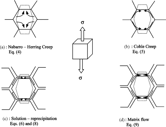
Fig. 3.34 A schematic representation of diffusion creep within crystals in response to an applied stress. As the vacancies move, the overall stress is lowered, and further macroscopic deformation occurs. There are several mechanisms by which vacancies can move, including diffusion through the crystal interior (Nabarro-Herring Creep) or along grain boundaries (Coble Creep). Figure taken from Bhadeshia (2003)

To gain further insight into the behaviour of a Maxwell solid, we can consider its response to a time-harmonic forcing. In this case, we can express the stress and strain as in the form

\[\sigma(t) = \tilde{\sigma} \mathrm{e}^{\mathrm{i}\omega t}, \quad \epsilon(t) = \tilde{\epsilon} \mathrm{e}^{\mathrm{i}\omega t}, \]

with \(\omega\) the oscillation frequency, and tilded terms the amplitudes. Note that the use of complex numbers is for convenience, and it is the real parts that are physically meaningful. Putting the above expressions into the governing relation for a Maxwell solid, we obtain

\[\tilde{\sigma} = \tilde{\mu}(\omega) \tilde{\epsilon}, \]

where we have introduced a frequency-dependent viscoelastic modulus

\[\tilde{\mu}(\omega) = \frac{\mathrm{i}\omega\tau }{\mathrm{i}\omega\tau + 1} \mu.\]

This shows that the constant of proportionality between the stress and strain amplitudes is both frequency-dependent and complex valued. The latter feature is associated with a phase delay between forcing and response, though this property is not crucial to our present discussion. It is this frequency-dependence, however, that makes precise the idea of a time-dependent rheology. In particular, we can now examine quantitatively the low and high-frequency limiting behaviour of a Maxwell solid.

High-frequencies are those for which \(\omega \tau \gg 1\), and in such cases we have the approximate relation

\[\tilde{\sigma} \approx \mu \tilde{\epsilon}, \]

this being identical to what would be seen within an elastic solid. Thus, when the material is deformed at a rate that is fast relative to the relaxation time, it behaves like an elastic solid. Conversely, at low-frequencies, we have \(\omega \tau \ll 1\), in which case

\[\tilde{\sigma} \approx \mathrm{i}\omega \mu \tau \tilde{\epsilon}. \]

Noting that \(\mathrm{i}\omega \tilde{\epsilon}\) is the amplitude of the strain-rate, we see that the behaviour is that of a Newtonian fluid with viscosity

\[\eta = \mu \tau.\]

More general viscoelastic rheologies

We have now shown that a Maxwell solid has the correct limiting behaviours seen within the Earth’s mantle. More detailed observations make clear that the mantle’s rheology is more complicated. Indeed, we noted above that within real crystals there will typically be a whole spectrum of relaxation times associated with different microscopic mechanisms. Nonetheless, the same form of low-frequency limiting behaviour of a Newtonian fluid can be expected under reasonable assumptions. To see this, suppose that the viscoelastic modulus for a Maxwell solid is generalised to

\[\tilde{\mu}(\omega) = \int_{\tau_{1}}^{\tau_{2}} \frac{\mathrm{i}\omega\tau }{\mathrm{i}\omega\tau + 1} m(\tau) \dd \tau, \]

with \(m(\tau)\) a function that quantifies the relaxation spectrum which we assume is limited to the range \(0 < \tau_{1} \le \tau_{2} < \infty\). We can then consider the low-frequency limit, meaning \(\omega \tau_{2} \ll 1\), for which we find

\[\tilde{\mu}(\omega) \approx \mathrm{i} \omega \int_{\tau_{1}}^{\tau_{2}} \tau m(\tau) \dd \tau, \]

and hence that the effective viscosity is given by

\[\eta = \int_{\tau_{1}}^{\tau_{2}} \tau m(\tau) \dd \tau.\]

Similarly, at high-frequencies, \(\omega \tau_{1} \gg 1\), such a material behaves elastically with effective modulus

\[\mu = \int_{\tau_{1}}^{\tau_{2}} m(\tau) \dd \tau.\]

This shows that the effective elastic modulus and viscosity can still be related by the simple expression

\[\eta = \mu \bar{\tau}, \]

where we have defined the average relaxation time

\[\bar{\tau} = \frac{\int_{\tau_{1}}^{\tau_{2}} \tau m(\tau) \dd \tau}{\int_{\tau_{1}}^{\tau_{2}} m(\tau) \dd \tau}.\]

It should be noted that the above discussion has been limited to linear rheologies. For sufficiently large strains or strain-rates, non-linear effects can be relevant and this is likely to be true for certain aspects of mantle dynamics. Accounting for such non-linearity adds complications to the above discussion, but does not alter the main points that have been emphasised.

Estimates mantle viscosity

An order of magnitude estimate on the relaxation time for the Earth’s mantle can be obtained through the study of glacial isostatic adjustment. This is the slow process of the Earth’s surface rising after the immense weight of an ice sheet is removed, much like a cushion slowly regaining its shape. This process is associated with the deformation of the solid Earth and concomitant sea level change associated with the growth or melting of large ice sheets. There is not time to enter into this process in any detail, but observations linked to the previous glacial period show that the relaxation time for the mantle is of order \(10^4\) years.

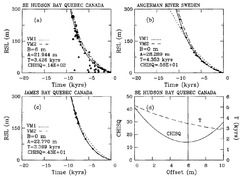
Fig. 3.35 Past sea level curves from locations under the centre of large ice sheets during the last glacial period. Since the ice has melted, these regions have undergone significant uplift, and hence sea level fall, due to viscoelastic relaxation of stress. The observed response can be well-modelled by an exponential decay, with the associated time-scale providing an estimate for the mantle’s Maxwell time of order 5000 years. Figure taken from Peltier (2004)

From our previous discussion, we know that mantle viscosity is related to the relaxation time through

\[\eta = \mu \tau, \]

with \(\mu\) an elastic modulus. An appropriate value for \(\mu\) can be obtained from seismological models for the Earth, with \(\mu \sim 10^{11}\) Pa being a suitable order of magnitude estimate. Recalling that one year is around \(10^{7}\) s, we find \(\eta \sim 10^{21}\) Pa s. For comparison, this is greater than the viscosity of water by twenty one orders of magnitude!

The study of glacial isostatic adjustment can also provide more detailed quantitative models of viscosity variations within the Earth. For example, it has been shown that the viscosity increases by between the upper and lower parts of the mantle by around one order of magnitude. Such a change in viscosity is likely due to solid-state phase changes within the minerals the make up the mantle, and both factors have potentially important effects on spatial pattern of convection. Such details are not, however, vital for our present discussion.

Temperature and pressure dependence of viscosity

The viscosity of the mantle is set principally by the relaxation time, with this quantity reflecting the aggregate effect of a host of microphysical processes. The relaxation time, and hence viscosity, is known to be a highly sensitive function of temperature, \(T\), and pressure, \(p\). This relation is complicated and not well-determined, but a reasonable model is given by

\[\tau = \tau_{0} \exp\left( \frac{E_{0} + p V_{0}}{k T}\right), \]

where \(E_{0}\) is a reference activation energy, \(V_{0}\) a reference volume, and \(k\) the Boltzmann constant. For those familiar with statistical mechanics, the form of this expression is motivated by the Boltzmann distribution, and reflects the fact that the microphysical mechanisms require energy barriers to be overcome, with the probability that this happens being higher and higher temperatures.

The strong temperature dependence of viscosity within the mantle is central to understanding the Earth’s interior dynamics along with related processes such as plate tectonics. As temperature decreases, relaxation time rises dramatically. Within sufficiently cool shallow parts of the Earth, the relaxation time can be so great that the material behaves elastically over geological time. This region of the Earth is called the lithosphere. It is known be around 100 km thick, comprising the Earth’s crust (which has an average thickness of about 35 km) and the upper part of the Mantle. It should be emphasised that the crust and mantle are compositionally distinct, with the former having, in broadest outline, formed through partial melting of the latter. The lithosphere, by contrast, is not defined in terms of its composition but from its long-term mechanical behaviour.

The Rayleigh number

While a full understanding of mantle convection is rather involved, the main ideas can be understood through simple scaling arguments. Convection in the mantle ultimately occurs because the Earth’s interior is hotter than its exterior, with this difference being due to a combination of heat generated during the Earth’s formation and that produced subsequently through radioactive decay.

Regions of the mantle that are hotter (colder) than their surroundings have lower (higher) densities due to thermal expansion and so they experience an upwards (downwards) buoyancy force. These buoyancy forces are resisted by the mantle’s viscosity. It can be shown – though analysis of the so-called Reynolds number – that the viscosity of the mantle is sufficiently great that accelerations are vanishingly small for mantle convection, and hence at each time there is a near perfect balance between buoyancy forces and viscous resistance to flow.

Heat can also be transfered within the mantle through thermal diffusion, with heat flowing from hot to cool regions without any bulk motion of the fluid. If the time-scale for thermal diffusion is much faster than that associated with fluid flow, then a thermal anomaly will diffuse away before any significant motion of the fluid can accumulate. This idea is quantified within the Rayleigh number that we now derive using a simple scaling argument.

Consider a region with characteristic length scale \(L\) that is temperature \(\Delta T\) hotter than its surroundings. Associated with this temperature difference, the region has a density anomaly

\[\Delta \rho = -\rho \alpha \Delta T, \]

where \(\rho\) is the background density, and \(\alpha\) is the thermal expansivity; the negative sign means that regions that are hotter, \(\Delta T > 0\), have a lower density, \(\Delta \rho < 0\), and conversely. The regions volume scales like \(L^{3}\), and hence the mass anomaly is

\[\Delta m \sim -\rho \alpha \Delta T L^{3}. \]

Here we write \(\sim\) and not equals to emphasise that this is just a rough estimate and not a precise equality. Finally, we multiply by the gravitational acceleration to arrive at the buoyancy force the region experiences

\[ F_{b} \sim -\rho \alpha g \Delta T L^{3}.\]

The bouancy force is resisted by the viscous resistance to flow. The viscous stress, \(\sigma = \eta \dot{epsilon}\), is a force per unit area, and so we can convert it to a force by multiplying by the boundary of the region whose area scales like \(L^{2}\):

\[ F_{v} \sim \eta \dot{\epsilon} L^{2}.\]

To proceed, we need to estimate the strain rate, \(\dot{\epsilon}\) for the fluid flow. The strain rate is a rate of change of velocity with distance, and so we have

\[ \dot{\epsilon} \sim \frac{V}{L}, \]

where \(V\) is the magnitude of the velocity and we assume that the scale-length for the flow is equal to the characteristic length-scale for the region. Combining with the above estimate we arrive at

\[ F_{v} \sim \eta V L. \]

We can now equate the magnitudes of the buoyancy and viscous forces to obtain

\[ \rho \alpha g \Delta T L^{3} \sim \eta V L, \]

and hence the flow speed scales like

\[ V \sim \frac{\rho \alpha g \Delta T L^{2}}{\eta}.\]

A time-scale can then be associated with the fluid-flow by setting

\[t_{a} \sim \frac{L}{V} \sim \frac{\eta}{\rho \alpha g \Delta T L}, \]

with sub-script \(a\) for advection.

Considering the same region, we can also estimate the time-scale over which is would cool by thermal diffusion. First, the total thermal energy associated with the region scales like

\[\Delta E \sim \rho C_{p} \Delta T L^{3}, \]

where \(C_{p}\) is a heat capacity (at constant pressure) measured per unit mass. If we write \(q\) for the heat flux (i.e., flow of energy per unit area per unit time), then to move all the heat from the region would take a time

\[t_{d} \sim \frac{\rho C_{p} \Delta T L^{3}}{q L^{2}} \sim \frac{\rho C_{p} \Delta T L}{q},\]

with subscript \(d\) for diffusion. To simplify further, we need to use Fourier’s law which states that the heat flux is proportional to the negative of the temperature gradient. This leads to the following scaling estimate for magnitudes

\[q \sim k \frac{\Delta T}{L}, \]

where \(k\) is the materials thermal conductivity. We can now simplify our expression for \(t_{d}\) to yield

\[t_{d} \sim \frac{\rho C_{p} L^{2}}{k} \sim \frac{ L^{2}}{\kappa}, \]

where in the final equality we have introduced the thermal diffusivity which is defined by

\[\kappa = \frac{k}{\rho C_{p}}.\]

We now have scaling estimates for the time-scales linked to advection, \(t_{a}\), and diffusion, \(t_{d}\), and combining these we arrive at the dimensionless Rayleigh number:

\[\mathrm{Ra} \sim \frac{t_{d}}{t_{a}} \sim \frac{\rho \alpha g \Delta T L^{3}}{\kappa \eta }\]

A key observation is that the Rayleigh number’s dependence on the length-scale goes like \(L^{3}\). This shows that relative importance of advection is larger for larger anomalies. It follows that if convective instabilities most readily occur at the largest possible length-scales.

A limitation of our simple scaling analysis is that we cannot know how large the Rayleigh number need be for the onset of convection. However, this quantity also occurs within a linearised stability analysis of the governing equations. There is not time to cover these details, but they show that when the Rayleigh number is larger than some critical value, \(\mathrm{Ra}_{c}\), convection will occur. The precise value depends on the geometry considered, but \(\mathrm{Ra}_{c} \sim 10^{3}\) is a representative value.

The above analysis can now be applied to the Earth’s mantle to assess whether it is likely to undergo convection. In doing this, it makes sense to choose the length-scale of the flow to be as large as possible, and so we take \(L\) to be the thickness of the mantle. Experiments on mantle minerals show that \(\alpha \sim 10^{-5}\) K \(^{-1}\) is an appropriate estimate. Determining a sensible value for \(\Delta T\), which can be viewed as the temperature difference from the bottom to top of the mantle, is more difficult. Instead, we will determine what temperature difference across the mantle would be required for convection to occur, and then consider if such a value seems plausible. Solving for \(\Delta T\) within the Rayleigh number, we find

\[\Delta T \sim \frac{\kappa \eta \mathrm{Ra}_{c}}{\rho \alpha g L^{3}} \sim \frac{10^{-6} 10^{21} 10^{3}}{10^{3} 10^{-5} 10^{1} 10^{18}}\, \mathrm{K} \sim 1 \,\mathrm{K}\]

Here we see that a temperature difference of order only one Kelvin would be sufficient for the mantle to convect! Given other geological information (volcanism, geothermal heat, radioactive heating) it is entirely implausible that the temperature difference across the mantle is smaller than this value, and hence convection must certainly occur.

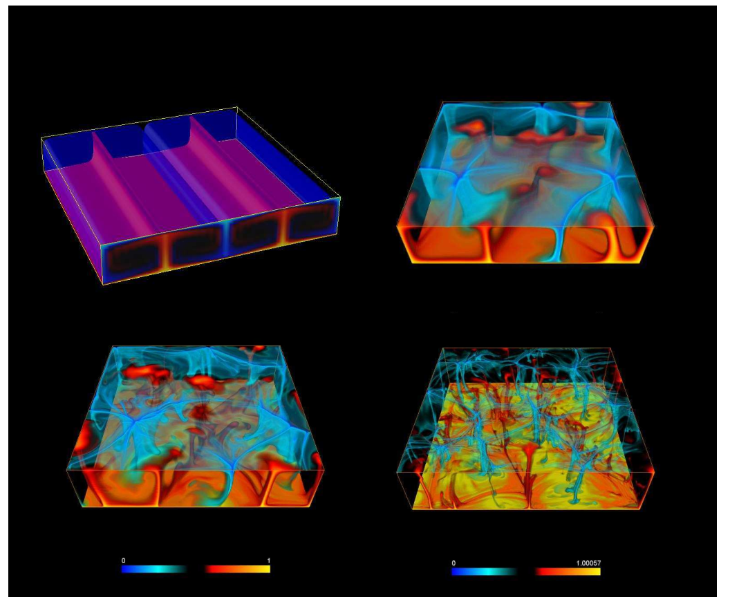
Fig. 3.36 Convection patterns of a fluid heated from below at Rayleigh number \(10^{3}\) , \(10^{6}\) , \(10^{7}\) , \(10^{8}\). The colour show non-dimensional temperatures. For the lowest Rayleigh number, lying just above the critical value, large scale convection cells form that undergo a quasi-steady flow. For larger values of the Rayleigh number, the convective patterns are more complicated, involve a range of length-scales, and are and strongly time-dependent. Figure taken from Ricard (2007).

In fact, plausible estimates for the mantle’s Rayleigh number are typically of order \(10^{6}-10^{7}\), and so around one thousand times larger than the critical value. At such high Rayleigh numbers, instabilities are not limited to the largest possible length-scales. Instead, complicated and time-dependent patterns of convection spanning a range of length-scales must occur.

Consequences of convection at the Earth’s surface

To conclude this lecture, we consider two consequences of mantle convection that are observable at the Earth’s surface, namely gravity anomalies and dynamic topography. These are not the only surface features linked to mantle convection, but most others on Earth are associated with to plate tectonics. Whether or not an Earth-like planet has plate tectonics, we would expect there to be gravity anomalies and dynamic topography linked to convection within its interior. Convection within the mantle is, however, not the only nor the dominant process that can produce gravity anomalies or topography on a planet’s surface, and hence there are significant challenges to using such observations in practice.

Gravity anomalies

If the Earth did not convect and if it was entirely fluid over geological time, then it would have an ellipsoidal equilibrium figure, with the surface being an equipotential of the gravity potential (i.e., the sum of the gravitational and centrifugal potentials). As we have seen, the lithosphere is sufficiently cool to behave elastically over geological time, with this layer supporting both topography and lateral density contrasts that have been generated by a host of processes. Moreover, convection within the mantle is driven by density anomalies whose gravitational signal can be felt at the surface,

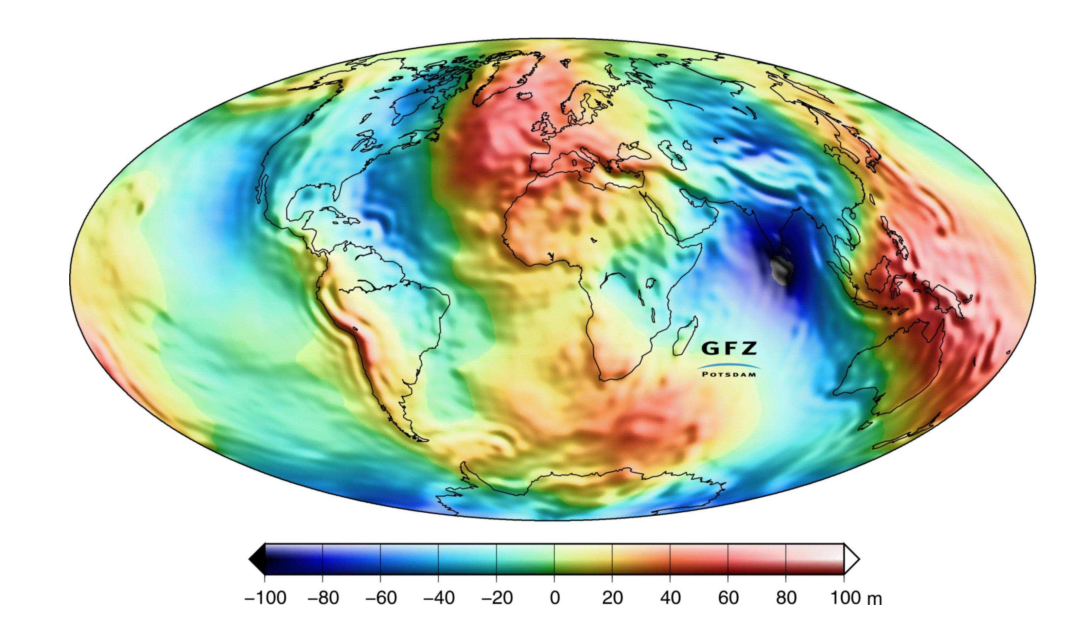
Fig. 3.37 Variations in the gravitational potential at the Earth’s surface expressed as the equivalent geoid anomaly. The latter quantity can be understood as the change in the position of the mean sea level associated with the gravitational potential perturbation. The observed geoid anomaly reflects contributions throughout the whole Earth, but it is only at the longest wavelengths that the effects of mantle convection can be seen.

Dynamic topography

Convection in the mantle applies a force at the base of the lithosphere. In areas of upgoing flow, the lithosphere, and hence the Earth’s surface, is deflected upwards, and conversely in areas of downgoing flow. The resulting topography at the Earth’s surface is known as dynamic topography, with this term being identical to that used within oceanography for deflections of the sea surface linked to large-scale ocean currents. Note that the deflection of the internal and external boundaries linked to mantle flow contributes directly to the associated gravity anomaly.

The elastic lithosphere acts as a low-pass filter on the forces applied to its base. As a result, dynamic topography is largest at long-wavelengths and is not appreciable at scales smaller than the lithospheric thickness. The amplitude of dynamic topography can be estimated using simple scaling arguments or through more sophisticated modelling. The result is that amplitudes of order 1 km might be expected at wavelengths of 1000 km.

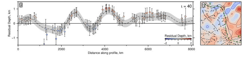
Fig. 3.38 Observations of dynamic topography for transect along the margin of Western Africa. These observations are obtained by correcting the observed topography for processes such as sedimentation. The amplitude of the dynamic topography is 1 km, and the horizontal wavelength is of order 1000 km. Figure from Holdt et al. (2022).

Observations of dynamic topography can be made on the Earth, but the process is complicated by the need to remove other sources of topography. This correction is significantly easier within the oceans, and as a result most observational models are limited to this region.

Further reading

• Turcotte, D.L. and Schubert, G., 2002. Geodynamics. Cambridge university press.

References

• Bhadeshia, H.K.D.H., 2003. Mechanisms and models for creep deformation and rupture.

• Holdt, M.C., White, N.J., Stephenson, S.N. and Conway‐Jones, B.W., 2022. Densely sampled global dynamic topographic observations and their significance. Journal of Geophysical Research: Solid Earth, 127(7), p.e2022JB024391.

• Peltier, W.R., 2004. Global glacial isostasy and the surface of the ice-age Earth: the ICE-5G (VM2) model and GRACE. Annu. Rev. Earth Planet. Sci., 32(1), pp.111-149.

• Ricard, Y., 2007. Physics of mantle convection. Treatise on geophysics, 7, pp.31-87.