2.1. Exoplanets I: Detection#
Professor: Amy Bonsor (IoA)
Learning objectives:
Methods of exoplanet detection and how they work
Radial velocity
Transit
Astrometry
Direct imaging
Microlensing
Key Concepts:#
exoplanets are generally detected by indirect methods, including radial velocity technique, transits, astrometry, direct imaging, timing and microlensing
Most of the Solar System planets, except Jupiter, lie beyond the capabilities of current methods
In general, close-in, massive planets are the easiest to detect, with a few caveats for individual methods
Transits#
The transit of a planet is detected when the planet passes directly in front of the star blocking light from reaching the observer. The observer luminosity of the star temporarily drops whilst the orbiting planet moves across the star, as shown in Fig. 2.1. The drop in the brightness of the star, or the flux received on Earth (\(F\)), is proportional to the area of the planet (\(R_{\rm pl}^2\)) relative to the area of the star (\(R_*\)):
\(F \propto \left (\frac{R_{\rm pl}}{R_*}\right)^2\).
Transits can be used to find the planet’s radius, given a good knowledge of the star’s radius. Transit photometry is best suited to detecting large planets on short period orbits around small stars. The probability of a planet transiting is proportional to its radius and inversely proportion to the semi-major axis of the planet’s orbit:
\(P \sim \frac{(R_* + R_{\rm pl})}{a}.\)
Fig. 2.2 shows that most planets detected by transits (blue dots) are on short periods and that transits can detect planets smaller than Earth, so long as they are orbiting small stars. This means that the first population of terrestrial mass planets have been found around stars significantly smaller than the sun, referred to as M-dwarfs.
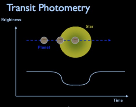
Fig. 2.1 A schematic showing the dip in brightness of the star as a planet passes in front.#
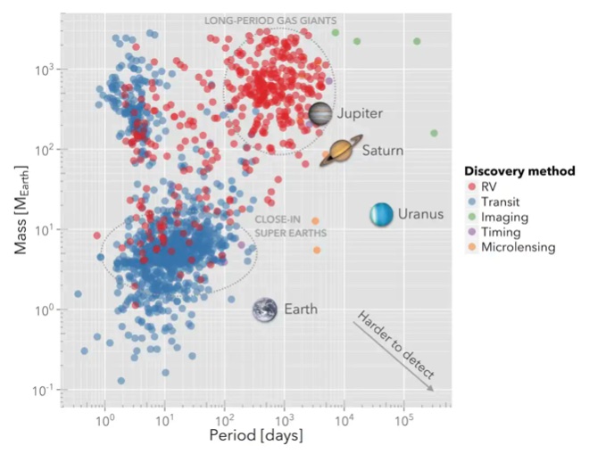
Fig. 2.2 The masses and periods of exoplanet detections shown, coloured by the primary discovery method. Credit: Stefano Meschiari.#
The Radial Velocity Technique#
Planets and stars both orbit the common centre of mass of the system. As the star is in general much more massive, the centre of mass is often very close to the star, such that the difference between the frame in which the planet orbits the star and the frame in which the planet orbits the centre of mass are very similar, as shown by Fig. 2.3. The orbit of the star around the planet-star centre of mass does, however, lead to small variations in the velocity of the star, as seen by an observer on Earth. The radial velocity detects this motion or wobble in order to infer the presence of a planet.
Stellar spectra contain a range of absorption lines from species in the stellar atmosphere. The exact frequency or wavelength at which these absorption lines are seen depends on the atomic properties of the line as well as the velocity of the star. If the star is moving towards the observer, the frequency of the emission increases. This is known as a Doppler Shift. As the star moves away from the observer, the frequency of the emission decreases. By following the variation in the frequency of a range of absorption features in the stellar spectrum, the radial velocity of the star as function of time can be tracked. The radial velocity of the star 51 Peg is shown in Fig. 2.4. The periodic change in the radial velocity is due to the star being orbited by a planet with minimum mass of 0.42 Jupiter masses on a 4.23 day orbit, as found by Mayor & Queloz, 1995.
The radial velocity technique is best suited to detecting massive planets on short period orbits, as shown on Fig. 2.2. Planets can be detected on longer period orbits, where the stars have been monitored on sufficiently long timescales. The technique provides the minimum mass of the planet, as for systems inclined to the line of sight to the observer, the observed radial velocity will be decreased by a factor of sin I, where I is the inclination of the planet’s orbit to the line of sight.
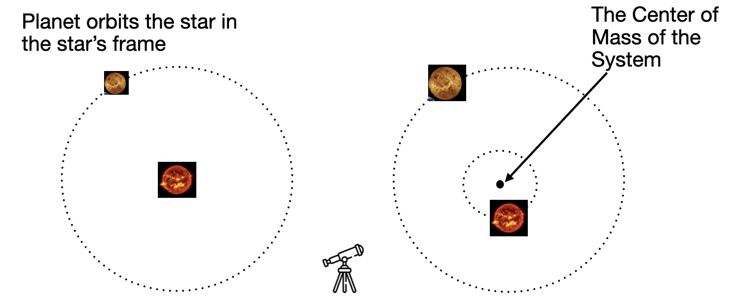
Fig. 2.3 As seen from Earth, both the star and planet orbit the common centre of mass of the system. In the star’s frame, the planet orbits the star.#
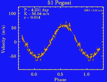
Fig. 2.4 The phase-folded radial velocity measurements for the plaent 51 Peg b (Mayor & Queloz, 1995).#
The radial velocity of a star is related to the trajectory of the star about the star-planet common centre of mass. If we consider the definition of the centre of mass, we can relate the orbital radius of the star, \(r_*\), to the planet-star separation, \(a\):
\( r_* = a \frac{M_p}{M_p + M_*} \),
where \(M_p\) is the planet mass and \(M_*\) is the stellar mass.
If the star is on a circular orbit, its velocity can be related to its period, \(P\) by:
\( v_*= \frac{ 2\pi r_*} {P}\),
which is simplified as:
\( v_*= \frac{ 2\pi a} {P}\frac{M_p}{M_* + M_p}\).
From Kepler’s third law:
\(a^3 = \frac{G(M_* + M_p) P^2}{4\pi^2}.\)
Thus, the stellar velocity can be expressed as:
\( v_* = \left ( \frac{2\pi G }{P}\right)^{1/3} \frac{M_p}{(M_* + M_p)^{2/3}}. \)
For an observer on Earth, who is inclined at an angle, \(I\) to the star-planet orbital plane, the observed velocity is \(v_* \sin I\). Including an eccentricity of the orbit, \(e\), the radial velocity semi-amplitude, \(K\) can be expressed as:
\( K = \left ( \frac{2\pi G }{P}\right)^{1/3} \frac{M_p \sin I }{(M_* + M_p)^{2/3}}\frac{1}{\sqrt{1-e^2}}\).
Astrometry#
Astrometry finds planets by precisely measuring the position of the star and looking for periodic shifts due to the orbit of the star around the common centre of mass for the planet-star system. The precision required to find planets is very high, however, the Gaia space mission is anticipated to find hundreds of exoplanets using astrometry.
The astrometric signature, \(\alpha\), is approximated by the ratio of planet and stellar masses (\(M_{\rm pl}\) and \(M_*\)) in solar masses, their separation, \(a\), and the distance to the star, \(d\) :
\( \alpha = \left (\frac{M_{\rm pl}}{M_*}\right) \left ( \frac{a}{\rm au}\right) \left (\frac{d}{\rm pc}\right)^{-1} \, \, as. \)
Astrometry is better suited to detecting higher mass planets on longer orbital periods, which is very complimentary to other techniques. However, multiple orbits still need to be observed in order to confirm a detection. The planetary orbit must also be face-on.
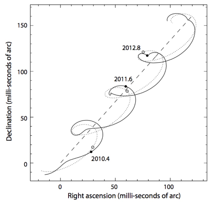
Fig. 2.5 The motion on the sky of a star due to its proper motion, parallax and orbital motion due to the presence of planet (Perryman et al, 2012). (European Physical Journal H, 37, 745 (2012))#
Direct Imaging#
Planets are very faint objects very close to their bright host stars. In general, it is very difficult to image them directly, unless they are very bright, normally the case only for young, massive planets and can be resolved from the star. Fig. 2.2 shows that the currently imaged planets orbit at tens of au from their host stars and our Jupiter mass and above.
Coronographs or star-shades can be used to block the light from the star, leaving the light from the planets that can be directly detected. The key advantage of direct imaging is that it is possible to get a spectra of the planet.
Fig. 2.6 shows an image of the planets found around the star HR 8799. This planetary system is very different to our Solar System with four planets more massive than Jupiter orbiting at tens of au.
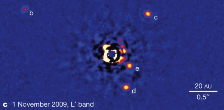
Fig. 2.6 HR 8799 b, c, d and e, Marois et al, 2010, Nature#
Timing#
The first exoplanets ever discovered orbited the pulsar, PSR B1257+12 (Wolszczan et al, 1992). Pulsars are extremely regular clocks and the variation in the arrival time of pulses indicated that the pulsar was orbited by 3 planets of 0.02, 4.3 and 3.9 \(M_\oplus\) on orbits with semi-major axis of 0.19, 0.36 and 0.46au.
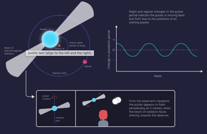
Fig. 2.7 Regular variations in the timing of pulses indicate the presence of a planet. Image credit: Alice Hopkinson, LCO.#