Macroevolutionary patterns on Earth

5.11. Macroevolutionary patterns on Earth#

Professor: Emily Mitchell (Department of Zoology)

Learning objectives:

Understand the key drivers that shape macroevolutionary patterns on Earth

Understand how the different forms of life have different interactions/impact on the biosphere

Introduction#

Macroevolution describes the evolutionary processes than have a large-scale taxonomic impact over geological timescales. The most common measures of macroevolution consider biodiversity, and how that changes through time. We can resolve macroevolutionary patterns through numerous routes, including the fossil record, geochemical record and with molecular and morphological phylogenies.

Null Models#

In order to consider what processes shape the evolutionary patterns that we see, we first need to consider what the null model is. The three main ways we can consider null models in an evolutionary context are through genetic drift, neutral molecular evolution and the unified neutral theory of biodiversity.

Organisms evolve through natural selection, whereby the fitness organisms will survive, and reproduce more, so the population (through time) will change such that the genes that make the organisms the fittest, i.e. the best adapted, will end up dominating, and through time, lead to speciation. Yet, through mechanisms of genetic drift, if by chance, more organisms with a certain trait or gene survive, then the relative proportions can change. This genetic drift is still evolution, but evolution due to random chance, not selection. Genetic drift impacts evolution by reducing genetic variation, which then potentially can reduce a populations ability to adapt to new changes or selection pressures. Genetic drift is particularly apparent in small populations, either due to small habitats or rare species. It can result in speciation, especially with small, isolated populations, known as peripatric speciation. Genetic drift feeds into the neutral theory of molecular evolution: for organisms with identical fitness (or indeed genotypes or traits with identical fitness), when reproduction occurs, there is a random shuffling of the genes. This random shuffling can change the frequency that genotypes that occur.

../../_images/GeneticDrift.svg — Fig. 5.57 A model of genetic drift. Credit: Samuel Velasco/Quanta Magazine: Neutral models#

Processes such as genetic drift happen on the very small spatial and temporal scale, and can be referred to as microevolution. It takes time for speciation, and indeed any sort of selection process to lead to large-scale or macroevolutionary patterns. One such metric to investigate such patterns is biodiversity, i.e. the number of species (or indeed general, families etc) through time. Understanding what leads to diversity is combines ecology and evolutionary studies. In ecology, the neutral theory of diversity was first hypothesized by Hubbell to describe patterns of diversity. The canonical point of view is that species adapt to their niches through selection, and so it is the difference between species that leads to the difference niche occupancy, that leads to diversity. In contrast, the neutral theory it is random chance that leads to the filling of niches, sometimes due to random death, then immigration, sometimes due to stochastic differences between leads to diversity.

Birth-death models are the most commonly used approaches for modelling diversification patterns. The simplest model just inputs two parameters: the extinction rate and origination rates, with the balance between them corresponding to the total turnover – high turnover means much greater origination than extinction and low turnover has high extinction rates than origination. Rates. At each point in time, and for each lineage there is a probability that the lineage will either go extinct or speciate. These birth-death models can reproduce slow diversification, followed by a rapid radiation which are consistent with macroevolutionary patterns of many major groups, such as arthropods and tetrapods.

Mass extinctions significantly change macroevolutionary histories, but the frequency, strength and cause of them varies in an unpredictable way. Mass extinctions tend to be selective, in that the sensitivity of organisms to mass extinctions will depend on the trait. After an extinction, generally there is a reduction in selection pressure as previously full niches become relatively open, and this often leads to a radiation post extinction. However the extent to which mass extinctions fundamental changed the nature of what was evolving, or just accelerated it is still very much debated.

../../_images/ecologicaldrift.svg — Fig. 5.58 A model of ecological drift. Credit: Samuel Velasco/Quanta Magazine: Neutral models#

Environmental drivers#

Niche models are ones where the environment (or sets of environmental variables) are determine species distributions through space and time, and can provide good models for macroevolutionary and macroecological patterns. Modern diversity shows distinct global patterns with diversity peaks around the equator, in a pattern know as the latitudinal diversity gradient (LDG). This LDG is largely driven by temperature, with the idea that warmer temperatures cause higher metabolism and mutation rates and shorter generation times, and so increase speciation rates. With higher metabolisms, come increased food demands, which potentially could then also increase competition and predator–prey interactions, leading to further speciation. The temperature dependence of speciation is also demonstrated through the strong correlations of diversity with mean world temperature in the fossil record.

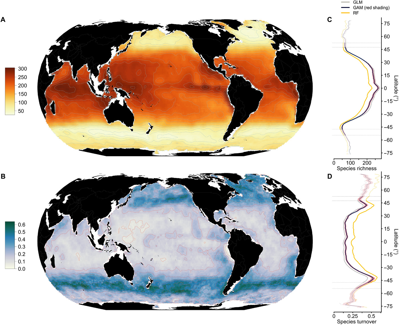
../../_images/climates.jpeg — Fig. 5.59 Global patterns of monthly phytoplankton species richness showing high diversity around the equator in and the tropics, with decreases towards the poles. Figure from Righetti et al. (2019).#

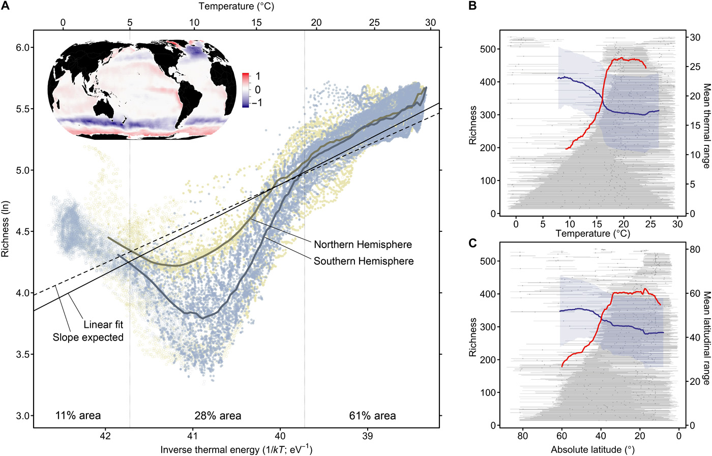
../../_images/LDG_offset.jpeg — Fig. 5.60 The relationship between species richness and temperature or latitude. The x-axis shows the sea temperature (inverse thermal energy, k, Boltzmann’s constant; T, temperature in kelvin), and the y-axis is the annual mean monthly phytoplankton species richness. The best fit polynomial regression models for the northern (green dots) and southern (blue) hemispheres against best-fit linear model (black line) values if richness was only a function of temperature, and the dashed line is the predictions from metabolic theory alone. Figure from Righetti et al. (2019).#

However, temperature doesn’t explain all the global diversity patterns we see in our oceans (see Fig. 5.59 and Fig. 5.60). Working out the relative importance of different contributing factors is hard because there is a lot of correlation and dependence between them, such as temperature with primary productivity. Primary productivity can increase diversity because high levels will produce more abundant populations, and thus drive speciation. Note that large-scale macroecological patterns can and do change through time. The LDG hasn’t always been present, originating around 15 million years ago (Fenton et al. 2023). The establishment of the modern-day LDG is consistent with a cooling climate that allowed for elevated higher rates of low-latitude speciation via niche partitioning at low latitudes, while restructuring distributions and removing niches at high latitudes.

Another key association of marine diversity is with the coastlines and the continental shelves. Generally species diversity and habitat diversity are intrinsically linked because in an area of low habitat diversity, the entire area may represent one habitat and thus the population range. In contrast, where habitat complexity is high, each habitat patch is separated by unsuitable habitat across which individuals must travel. Any migrants across unsuitable habitat risk high mortality due to environmental stress, lack of food, or predation. Animals adapt to this risk in different ways they can be small and use passive dispersal to save energy, being so large and fast as to minimise predation, or migrating at night to avoid visual predators. Thus, greater habitat heterogeneity will increase spatial separation of sub-populations, as well as opportunities for sub-populations to adapt to different microhabitats, and consequently the opportunity for speciation.

A connected idea, is that through geological time global biodiversity is influenced by tectonically driven shifts in the arrangement of continental crust, because diversity is high on the continental shelves, so the extent of the shelf areas will correlate with diversity. In terms of global marine biodiversity over the last 540 million years, there is a positive correlation between global marine invertebrate genus richness and an index of the fragmentation of continental crust during super continental coalescence–breakup cycles (Zaffos et al. 2017). Note that because many different environmental and biotic factors may covary with changes in the geographic arrangement of continental crust, it is difficult to identify a specific causal mechanism.

Taken together, these examples illustrate that there isn’t a single causal factor for global biodiversity patterns, it is a combination of many different factors which include temperature, primary productivity patterns and habitat complexity, and how those then impact the biotic interactions of animals.

Biotic Drivers#

While environmental or niche models can explain many macroevolutionary patterns, it is the interactions between organisms that leads to natural selection. One way to see the impact of biotic interactions is to consider how biogeographical patterns change through time. These are important not only ecologically over shorter timescales, but also over longer time scales because geographic range is a very strong predictor of how likely an species is likely to extinct – if it only lives in a very small area, and that area is disturbed, it will die out. But if the same species occupies many different areas, then not only can they survive, but they can also repopulate. Biogeographical patterns are strongly predicted by environmental conditions, such as temperature, but there are also strong drivers in the form of biotic interactions. These include competition for food, for suitable habitat, as well as indirect competition, predator prey interactions, and parasite host interactions. The impact of competition can be seen with the biographical patterns of pumas and leopards. Currently pumas are restricted to the new world, and leopards are found in Africa and Asia now, but historically pumas were also in Eurasia. As leopards got more successful, expanded up into Europe, and drove the pumas to extinction there, outcompeting for very similar prey.

In terms how these biotic and abiotic factors change over time. For marine taxa over the last 540 million years diversity there were two different timescale-dependent regimes with a crossover 40 million years. For shorter timescale diversity correlated with the palaeotemperatures, whereas for longer timescales origination and extinction rates and their magnitudes become highly correlated with diversity. Over these longer timescales they also strongly negatively correlated with standing diversity levels, indicating biotic drivers. Together this demonstrates that short time changes in diversity are driven by temperature, and longer term diversity changes are driven by biotic interactions.

While we have discussed evolutionary drivers in terms of null or stochastic models, environmental and biotic interactions, of course they can and often all work together. The combination can be seen after the Permian-Triassic mass extinction. This mass extinction was triggered by volcanism (so stochastic/random) but afterwards there is a radiation in predation, and a shift of ecosystem structure. One possible driver for these novel predatory adaptation is the breakup of Pangea (the supercontinent), which formed new oceans as it broke up, bringing together previously isolated marine communities. There was also an increase in habitat complexity, creating more niches so likely diversity.

Biosphere Impacts#

For life to persist, that is the biosphere needs to be relatively stable over geological timescales. The source of this stability can come through the environment and abiotic stabilising feedbacks and/or biotic feedbacks. Prior the evolution of animals the main stabilising forces environmental, and while life had a substantial impact on the biosphere, through the creation of oxygen for example, the ability of life to correct for any perturbations was quite limited. However, that changed with the advent of animals, and then with land plants and humans. Animals changed the biosphere because they could adapt their own habitat to make it more suitable for themselves and other life and be able to respond and correct much larger perturbations within the ecosystems. More broadly if we look at the major transitions where life changed the biosphere, they were all different. First, with the origins of life, and then with the originations of oxygenic photosynthesis, animals, and their ecosystem engineering, before land planets terraforming the terrestrial continents.