4.6. Atmospheric Chemistry I

Professor: Alex Archibald (Yusuf Hamied Department of Chemistry)

---

In these two lectures I aim to cover the basic physical chemistry that controls the reactions that can happen in an atmosphere.

Our starting point is that atmospheric composition plays an important role in providing the environment for life to emerge and thrive. Our questions are then, what determines the composition of an atmosphere (covered through C1 and C2) and how and why does that composition change over time (covered herein).

Key Concepts:

• To calculate and understand how to interpret the lifetimes and timescales of species in an atmosphere

• To understand what role thermal kinetic processes play in an atmosphere.

• To understand the role of photochemical processes and how they arise in an atmosphere.

• To build and simplify complex reaction networks.

Atmospheric composition change

It’s quite obvious to think about understanding how the composition of an atmosphere changes over time, but other than the last few decades, we have limited direct evidence. We do have a wealth of data on the vertical profile of atmospheric composition and we will come back to what this is telling us through the lectures.

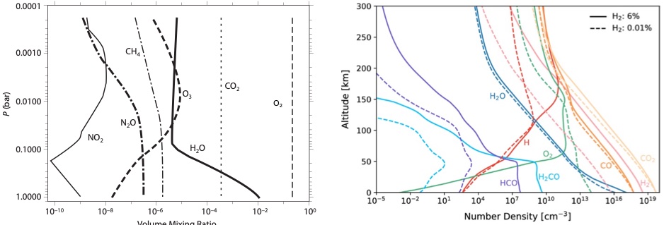
Fig. 4.52 Vertical profile of atmospheric gases in Earth’s modern atmosphere (left) expressed as volume mixing ratios (Seagar 2010) and of early Mars expressed (right) in number density (Koyama et al., 2024).

Time scales and lifetimes

As students of atmospheric chemistry we are fundamentally interested in understanding how the constituents of an atmosphere (the gases and particles that make it up) change with time. In order to understand this we rely on a solid knowledge of firstly what is in the atmosphere (the composition) and secondly how the constituents in the atmosphere react over time (the reaction network). Hence, it’s fair to say that chemical kinetics is at the heart of atmospheric chemistry.

For simple chemical systems, we can write out differential equations that describe how the components of the system will change over time. Let’s start with a trivial example. Suppose that we study in a closed constant-volume system a reaction whose rate depends on the concentration of one reacting substance, A, only. We can write,

\[ \frac{d[{\rm A}]}{dt} = -k[{\rm A}]^n \]

where in this case n = 1 and this reaction is said to be first-order with respect to A (molecules cm\(^{-3}\)) . Plots of the change in concentration of A with time are shown in Fig. 4.53 for different values of rate coefficient, k (s\(^{-1}\)). Fig. 4.53 highlights that the larger the value of the rate coefficient (sometimes called rate constant and erroneously as the rate - naughty!) the faster the loss of A with time.

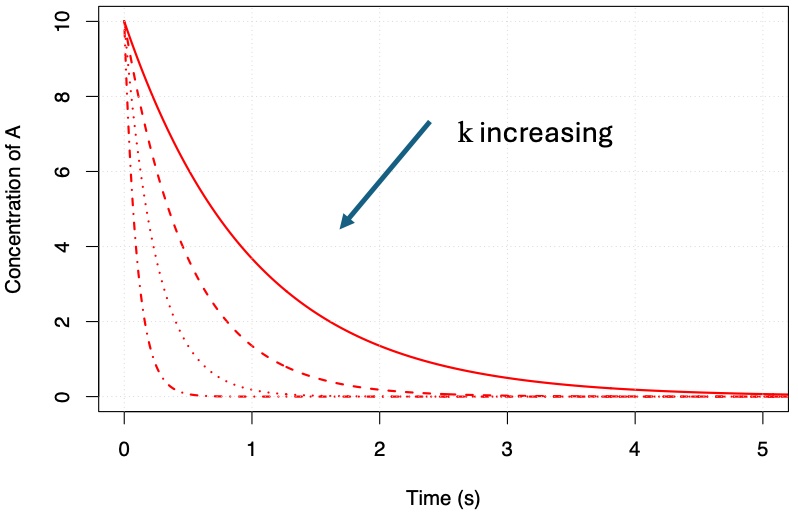
Fig. 4.53 Plots of the first order decay of [A] with respect to time.

We can define a new expression by integrating our rate equation for A and noting that our initial conditions are \(A = A_0\) at \(t = 0\):

\[ \int_0^t k \, dt = - \int_0^{\rm A} [{\rm A}]^{-n} \, d{\rm A} \]

Given that \(k\) and \(n\) are constants we can then write:

\[ [{\rm A}]_t = [{\rm A}]_0 \exp\big(-kt\big) \]

Or:

\[ [{\rm A}]_t = [{\rm A}]_0 \exp\big(-t/\tau) \]

As Fig. 4.53 highlights, the decay of A with time can be described as a simple exponential process. We can use this graph and the equations above to define the time constant (\(\tau\)) as the time taken for the concentration of A to be reduced by \(1/e^{\rm th}\) of its value.

\[ \tau = 1/k \]

The smaller this time constant the greater the loss of A with time and hence the shorter its lifetime.

In an atmosphere there are many very important reactions that are first order and, fortunately, many that can be described as pseudo first order. For example, consider the slightly more complex reaction:

\[ {\rm A + B} \xrightarrow{k_2} {\rm C} \]

On first glance we expect this to be a second order process (first order in A and first order in B so second order overall). However, if the concentration of [B] doesn’t change much over time (for example because B is present in large excess relative to A) then we can make the approximation that \(d[B]/dt \simeq 0\), which allows us to consider A as undergoing pseudo-first order kinetics ([B] \(\sim\) constant and so it can be folded into our second order rate constant (\(k_2\)) to yield a pseudo-first order rate constant, \(k_2’=k_2[{\rm B}]\)). The time constant for A is now given by:

\[ \tau = \frac{1}{k_2[{\rm B}]} = \frac{1}{k_2'} \]

We will now consider a slightly more complex example but one which you may be familiar with. Let’s consider the chain reaction:

\[ {\rm A} \xrightarrow{k_1} {\rm B} \xrightarrow{k_2} {\rm C} \]

where A is our initial reactant, B an intermediate product and C the final product of the reaction. Following the same procedure as above we can write:

\[\begin{split} \begin{align} \frac{d[{\rm A}]}{dt} &= -k_1 [{\rm A}] \\ \frac{d[{\rm B}]}{dt} &= k_1 [{\rm A}] - k_2 [{\rm B}] \\ \frac{d[{\rm C}]}{dt} &= k_2 [{\rm B}] \end{align} \end{split}\]

Solutions for these equations are shown in Figures Fig. 4.54 and Fig. 4.55.

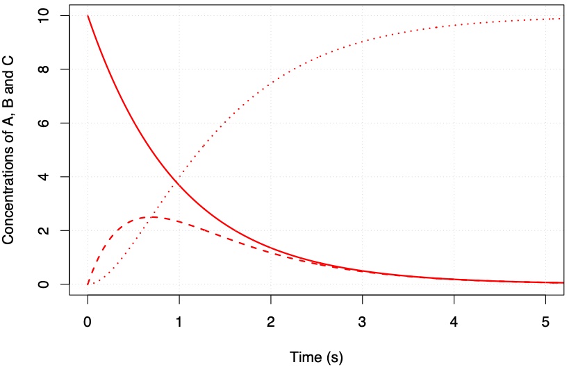
Fig. 4.54 \(k_1 = 1\) s\(^{-1}\) and \(k_2 = 2\) s\(^{-1}\).

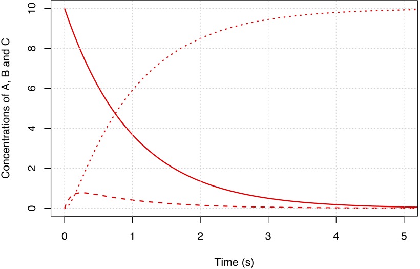
Fig. 4.55 \(k_1 = 1\) s\(^{-1}\) and \(k_2 = 10\) s\(^{-1}\).

What you will notice from the figures above is that the intermediate B is short lived relative to C and that as the value for \(k_2\) increases the peak concentration of B decreases. The time it takes for B to reach an almost steady concentration is \(\sim 1/k_2\). In the limit where \(k_2 \gg k_1\) we can make the approximation:

\[ \dfrac{d[{\rm B}]_{ss}}{dt} \simeq 0 \]

where the subscript \(ss\) is used to note that we are considering the intermediate B to be in steady state.

Following this through, we can re-write the remaining equations which describe our complex reaction (making the substitution \([{\rm B}]_{ss}=k_1 [{\rm A}]/k_2\)):

\[\begin{split} \begin{align} \frac{d[{\rm A}]}{dt} &= -k_1 [{\rm A}] \\ \frac{d[{\rm C}]}{dt} &= k_2 \times \frac{k_1 [{\rm A}]}{k_2} \simeq k_1 [{\rm A}] \end{align} \end{split}\]

In doing so we have greatly reduced the complexity of this reaction system.

In an atmosphere there are many examples of compounds that can be considered to be in steady state. In general a good opening argument to decide whether or not to put something into steady state is to consider whether or not it is a radical. For the steady state assumption to apply it is necessary that the intermediates that are involved to have rates for their destruction that greatly exceed those for their formation so that their concentrations remain low and constant over time.

Often we can consider the concept of an air parcel. An air parcel can be thought of as a “box of air”. Hence, we can consider what the inputs into the box are and what the outputs are.

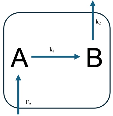
Fig. 4.56 Schematic showing possible connections between an A and B molecule with A undergoing emission.

We can appeal to steady state and write out steady state solutions for [A] and [B]

\[\begin{split} \begin{align} \frac{d[{\rm A}]}{dt} &= F_A - k_1 [{\rm A}] - k_2[{\rm A}] \\ [{\rm A}]_{ss} &= \frac{F_A}{k'} = F_A \times \tau_A \\ \frac{d[{\rm B}]}{dt} &= k_1 [{\rm A}] - k_2[{\rm B}] \\ [{\rm B}]_{ss} &= \frac{k_1[{\rm A}]}{k_1} \end{align} \end{split}\]

And we can then write an expression for the ratio of \([{\rm B}]_{ss}/[{\rm A}]_{ss}\)

\[ \dfrac{[{\rm B}]_{ss}}{[{\rm A}]_{ss}} = \frac{k_1}{k_2} \]

In other words, the ratio of B:A will depend on the magnitude of the rate constants \(k_1\) and \(k_2\) – which determine the lifetimes of A and B.

Finally, we can integrate our expressions for \(d[{\rm A}]/dt\) and with the boundary condition that [A]\(_0\) and \(t_0 = 0\) show that:

\[ [{\rm A}]_t = \frac{F_A}{k_1}\Big(1 - \exp(-k_1t)\Big) \]

or

\[ [{\rm A}]_t = F_A\tau_A \Big(1 - \exp(-k_1t)\Big) \]

So here we can see that the [A] will tend to the first term on the RHS as the system tends to infinity. In other words, when we consider a system with emissions (or a constant rate of production) then the concentration of A will be determined by the lifetime of A and the magnitude of the emission.

Note, that for a system of two first order (or pseudo first order) reactions:

\[ {\rm A} \rightleftarrows {\rm B} \]

With rate constants:

\[\begin{split} \begin{align} {\rm A} &\xrightarrow{k_1} {\rm B} \\ {\rm B} &\xrightarrow{k_{-1}} {\rm A} \end{align} \end{split}\]

the system approaches equilibrium with a time constant of \((k_1 + k_{-1})^{-1}\) (s). So, only need \(k_1\) or \(k_{-1}\) to be large for \(\tau\) to be small, and to then allow us to apply steady-state.

So far we have considered some very trivial examples. Whilst these have been trivial, they are still very useful for our studies of atmospheric chemistry. But an important complication for us as atmospheric chemists is that the reaction vessel we use in our studies is an atmosphere itself! You only need to venture outdoors to note that the reactions that are taking place in Earth’s atmosphere are doing so under far from controlled conditions! The gases and particles that we are interested in are affected not only by chemical change but also transport – for example through the wind. We won’t dwell much on atmospheric transport. What is important, however, is to have a feel for the relative time scales of chemistry and transport.

One way of doing so is to consider the major types of transport and their causes. These are hard to define universally – as things like tidal locking of a planet can lead to differences in atmospheric circulation but roughly they encompass:

• turbulent diffusion (fast, timescales of seconds to minutes to travel 10-100 m, caused by thermal instability or mixing over rough terrain – random)

• zonal mixing (transport along lines of longitude, usually fast – order of minutes to days to travel kms)

• meridional mixing (slow, timescales of days to months to travel kms, caused by thermal gradients from differential heating)

• Vertical mixing (typically slow, days to years to travel kms, but dependent on the lapse rate of the atmosphere – the change in temperature with altitude)

Before we go on to examine the role of atmospheric photochemistry on the composition of an atmosphere we will briefly review the forms of rate coefficients for gas phase reactions.

Bi-molecular rate coefficients (thermal)

Elementary reactions that involve two constituents can be written as:

\[ {\rm A + B} \xrightarrow{k_{\rm obs}(T)} {\rm products} \]

Often it’s found that the rate coefficients for these types of reactions observe temperature dependence. Whilst we can use tools like quantum mechanics and statistical thermodynamics to predict the rate constants and their temperature dependence, in this course we will just be making use of experimentally (observed) data.

Second order, or bi-molecular, rate coefficients are usually expressed using the following form in atmospheric chemistry:

\[ k_{\rm obs}(T) = A \times \exp\Bigg(-\frac{E_a}{RT}\Bigg) \;\; ({\rm molecules^{-1} \; cm^3 \; s^{-1}}) \]

where \(A\) is often referred to as the Arrhenius pre-exponential factor, \(E_a\) the reaction activation energy (J mol\(^{-1}\)), \(R\) the gas constant (J K\(^{-1}\) mol\(^{-1}\)) and \(T\) temperature (K). Many bi-molecular reactions exist in the atmosphere and many of these show temperature dependence in their kinetics. A good example is the reaction of OH with methane (CH\(_4\)) (one of the most temperature dependent reactions known).

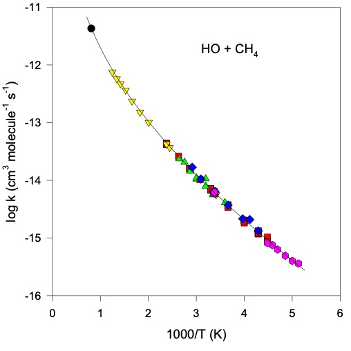
Fig. 4.57 Arrhenius plot for the reaction between methane and the hydroxyl radical in the gas phase.

Fig. 4.57 demonstrates that the reaction OH + CH\(_4\) proceeds with a significant activation energy barrier. By temperature we can think of the thermal energy of our gases (\(RT\)). As temperature is decreased there will be a lower fraction of reactants that can overcome this barrier and hence the observed rate of reaction will be decreased.

Termolecular Rate Coefficients

A more complex but fairly common type of reaction that is of interest in the atmosphere is the reaction between two compounds in the presence of a third body:

\[ {\rm A + B + M} \xrightarrow{k_{\rm obs}(T)} {\rm products} \]

Strictly speaking most reactions require a third body (often referred to as M) to remove excess energy from the initial reaction. Consider the reaction between two Iodine atoms. When the two atoms come together to form an iodine molecule, energy equal to the bond dissociation energy of I\(_2\) is released into the nascent molecule. This is enough energy to then rupture the I-I bond and thus reform the iodine atoms. However, if the nascent I\(_2\) molecule (I\(_2^*\)) is involved in a collision with a third body the encounter can transfer some of the vibrational and rotational energy of the I\(_2\) molecule to translational (and other) excitation of the third body.

\[ {\rm I + I} \rightleftarrows {\rm I_2^*} \xrightarrow{{\rm M}} {\rm I_2} \]

Under Earth’s atmospheric conditions, M is usually N\(_2\) or O\(_2\) and to a first order can be considered as the sum of their concentrations ([M] = [N\(_2\)] + [O\(_2\)]). For other atmospheres M will be the sum of the mixing ratios of all the gases present. The ability of the third body to “quench” the reaction to products depends on the structure of the third body. Generally speaking polyatomic quenchers (e.g., H\(_2\)O or CO\(_2\)) are “better” than mono-atomic species. The rate coefficients for ter-molecular reactions can be experimentally determined as a function of temperature and pressure to derive the low-pressure limits (\(k_{0,T}\)), which show pressure dependence and high-pressure limits (\(k_{\infty,T}\)) which don’t. In order to predict the observed rate constant as a function of temperature and pressure we need to combine these two limits using the Troe equation (a modification of the Lindemann-Hinshelwood expressions), which yields a pseudo bi-molecular rate coefficient:

\[ k_{\rm obs(M,T)} = \Bigg(\frac{k_{0,T}[{\rm M}]}{1 + \frac{k_{0,T}[{\rm M}]}{k_{\infty,T}}}\Bigg) F\Bigg\{1 + \Bigg[\log_{10}\Big(\frac{k_{0,T}[{\rm M}]}{k_{\infty,T}}\Big)\Bigg]^2\Bigg\}^{\!\!-1} \; \; ({\rm molecules^{-1} \; cm^3 \; s^{-1}}) \]

Kinetics as a guide to mechanisms

We can also use studies on the kinetics of chemical reactions to tell us about their mechanisms. By mechanism we mean the elementary series of steps (or step) involved in a molecular encounter. An example is the oxidation of the aromatic compound, benzene. The main sink for benzene is the reaction with OH. OH can either add to the aromatic ring on benzene or abstract (pull off) a hydrogen atom.

\[\begin{split} \begin{align} {\rm OH + C_6H_6} &\xrightarrow{k_1} {\rm H_2O + C_6H_5} \\ {\rm OH + C_6H_6} &\xrightarrow{k_2} {\rm HOC_6H_6} \\ k_{{\rm obs},T} &= k_1 + k_2 \end{align} \end{split}\]

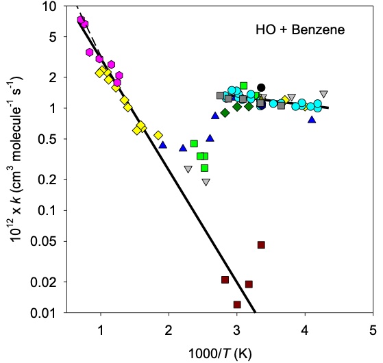
Fig. 4.58 Arrhenius type plot for the reaction between benzene and the hydroxyl radical in the gas phase.

Fig. 4.58 shows that the kinetics for the reaction between OH and benzene are complex! We can use the Arrhenius plot to infer that there is a change in mechanism for the reaction as a function of temperature. By doing analysis of the products of the reaction we see that at lower temperatures the hydroxyl radical adds to the benzene ring and at higher temperatures the hydroxyl radical abstracts one of the benzene hydrogen atoms. This is just an example of the complexity at play in an atmosphere.