Introduction to the core course

Course Director: Oliver Shorttle (IoA, Department of Earth Sciences)

---

The core courses follow a narrative arc, from the formation of planets (C1), through to the establishment of habitable environments (C2), how the chemistry of water and atmospheres on planets might enable life to arise (C3), and, finally, to life as an ecological and planetary scale phenomenon (C4).

We will motivate the structure of the core course by here considering the Drake equation, that famous expression of how likely we are to find life in the Universe.

Learning objectives from the Core Course:

• Gain a fluency in the key topics relevant to planetary science and life in the Universe from across disciplines. In particular:

  • The key processes forming planets;

  • The important processes maintaining planetary habitability;

  • The astrochemistry and geochemistry that gave rise to life and might enable us to detect it on planets; and,

  • How life operates at scales from the chemical to the ecological to shape environments.

• The multitudinous factors, from the Universe’s physical constants to whether a planet has a moon, that life’s emergence may be contingent upon.

Learning objectives: Core course introductionx

• The formulation of the Drake equation (Drake, 1965).

• How parameters in the Drake equation have been and can be constrained, and the assumptions required to find these constraints.

• The limits of the Drake equation’s use.

The Drake equation

The Drake equation is:

(1.1)\[N_c = R_* \cdot f_p \cdot n_e \cdot f_l \cdot f_i \cdot f_c \cdot L,\]

where \(N_c\) is the mean number of communicative civilizations in the galaxy, \(R_*\) is the rate of start formation, \(f_p\) is the fraction of stars hosting planets, \(n_e\) is the mean number of planets per start capable of supporting life, \(f_l\) is the fraction of those potentially habitable planets on which life emerges, \(f_i\) is the fraction of those inhabited planets where intelligence develops, \(f_c\) is the fraction of ‘intelligent’ civilisations that develop communication, and \(L\) is the mean communication timescale.

Now, many legitimate criticisms have been levied against the Drake equation (e.g., Alm’ar, 2011; Smith, 2011). However, this expression remains useful for at least two reasons. First, as an example of how we might like to combine insights from across disciplines to address a common and fundamental question; in this case, the likelihood of receiving communications from other intelligent life in the galaxy. Second, it focusses attention on what we need to know to better understand our chances of success in searching for life. Both of these principles are at the heart of the PSLU course.

Importantly, the specific parameters the Drake equation includes are, unlike when Drake first wrote down the equation, now partially constrained by observation. We therefore know better than ever before at least some of the relevant information to predict life’s prevalence in the galaxy.

In this section we summarise some of what we know about the parameters of the Drake equation, which from left to right map conveniently onto our Core Course journey from astrophysics, Earth sciences, chemistry, through to biology.

\(R_*\), the mean rate of star formation

This is the first parameter in the Drake equation and the first to have a reliable estimate. The key to our knowledge of this parameter is that it is a direct observation of stars, and unlike planets, stars are bright (see Fig. 1.2 for a comparison between the light emitted from solar system planets compared to the Sun).

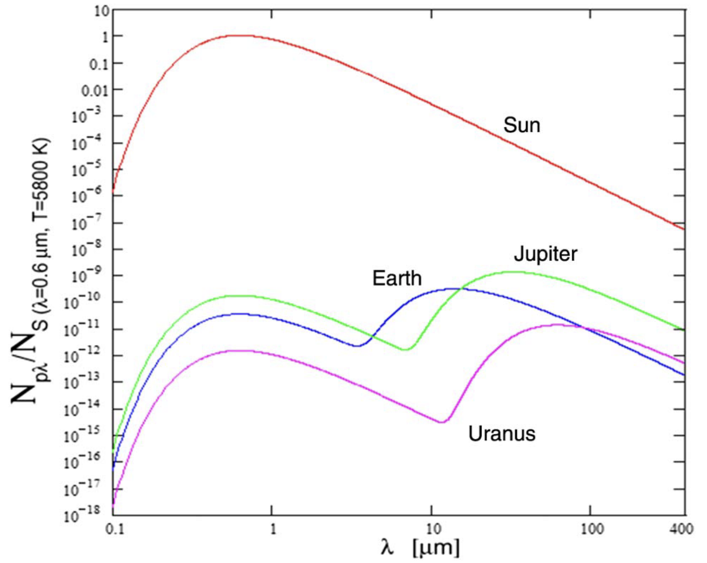
Fig. 1.2 A spectra showing the relative flux (of photons) coming from the Sun and solar system planets. Across the spectrum, the Sun is at least 4 orders of magnitude brighter than the solar system planets, and in the case of Earth nearly 10 orders of magnitude brighter. This represents the fundamental challenge to direct observation of Earth-sized planets around other stars: the light of the planet is overwhelmed by the light coming from the star. Credit: Galan+2016.

The rate of star formation can be estimated from the brightest stars. The brightest stars are large, with high surface temperatures (called ‘O or B’ type stars in stellar classification). Importantly, these stars have short lives, possibly of only a few tens of millions of years. This is in contrast to what will be the Sun’s approximately 10 billion year lifetime. As a result, these high-mass stars will be present only in galactic regions actively forming stars. Their brightness makes them the easiest to observe, even when in other galaxies. So, we can use massive stars to probe the rate of formation in our galaxy and beyond, provided their rate of formation can be linked to the rate of formation of lower mass stars – if we can do this, then the total rate of star formation can be estimated. This link between stellar occurrence rate and mass is known as the ‘initial mass function’ (Fig. 1.3).

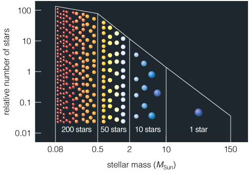
Fig. 1.3 A representation of the ‘initial mass function’. Smaller stars are significantly more abundant that larger stars in the galaxy. Credit: LASP, U Colorado Boulder.

With confidence that you can extrapolate from massive stars to the frequency of (the more nuerous) lower mass stars with the initial mass function, then massive stars allow star formation rates to be estimated in the galaxy and even in distant galaxies. Fig. 1.4 illustrates this beautifully, with the bright blue regions of the Antennae galaxies recording the birth environment of tens of thousands of new stars

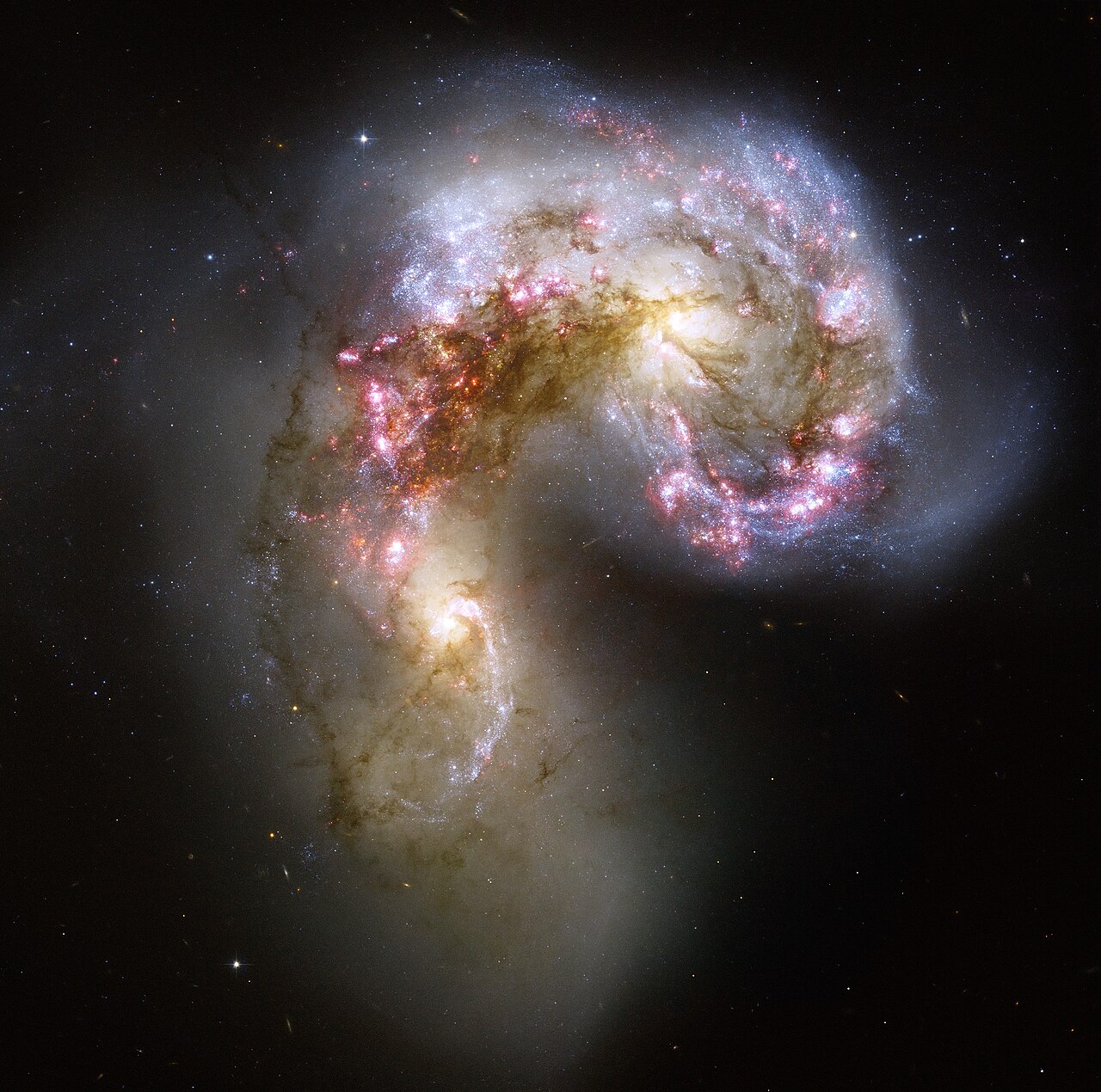
Fig. 1.4 The Antennae galaxies imaged by the Hubble Space Telescope. These galaxies are undergoing merger, triggering massive star formation. These areas show up as blue in these images, as they are illuminated by young massive and short lived O/B stars. In contrast, the two older regions show up as orange in these images, hosting older and cooler stars. Credit: NASA, ESA, and the Hubble Heritage Team (STScI/AURA)-ESA/Hubble Collaboration.

In summary then, the rate of star formation is something that we can see in our own galaxy today and even observe in distant galaxies. Given the star formation rate affects the gross spectral properties of a galaxy, it is something we can even then reconstruct going back in time through the history of the Universe, as we look to more distant, and therefore older, galaxies. C1 ‘The origins of planets’ will go into more detail on these topics.

\(f_p\), the fraction of stars hosting planets

For a long time the fraction of stars hosting planets was completely unknown. This picture was overturned first with the discovery of planets around a neutron star (Wolszczan & Frail, 1992), and then with the discovery of a Jupiter mass planet orbiting a main sequence star (Mayor & Queloz, 1995). However, it was some time later before good statistics were obtained on the occurrence of planets around stars. Even today, the limitations in sensitivity of our observation methods mean we cannot provide reliable estimates for the occurrence rate of all planets around all types of star: overall, our surveys are biased to discovering shorter period planets, that are more massive, around smaller stars. Earth itself, orbiting a G type star, remains a challenge to discover with current technology, and hence to quantify the frequency of.

Nonetheless, we now know planets are extremely common. Fig. 1.5 is a recent summary of discovered exoplanets, of which there are now over 5000.

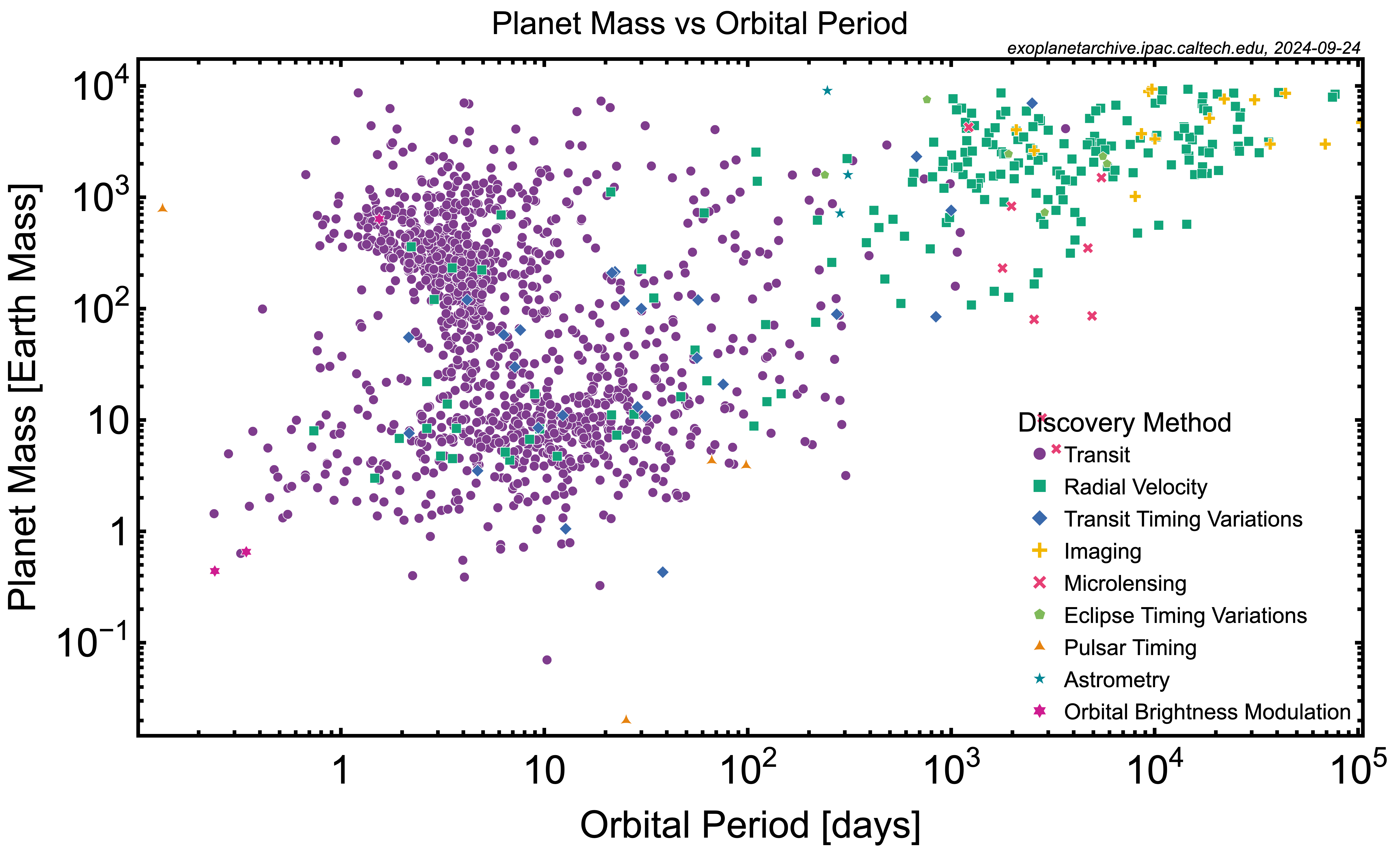
Fig. 1.5 Here we see the distribution of discovered exoplanets, coloured according to discovery method. Looking to the 1 Earth mass - 1 earth year portion of the diagram, you can see there is a sparsity of data, reflecting limitations of observation rather than a known dearth of planets. Conversely, massive planets are present in this plot far in excess of their occurrence rate in nature. You can try making these plots yourself through the NASA exoplanet archive. Credit: NASA exoplanet archive.

Fig. 1.5 does not in and of itself tell us about the planet occurrence rate – although many stars have been observed for signs of accompanying planets, we need to be fortunate for the planet to show up in the star’s light (see C1 ‘The origins of planets’ for more information on planetary detection methods). Instead, statistical extrapolation is required from the discovered population to the true underlying population. This is possible because many of the factors dictating whether a planet is discovered or not are well understood.

Accounting for these biases in discovery, plots such as Fig. 1.6 can be produced. If we are simply interested in the occurrence rate of planets of any sort around stars, then this plot suggests that it is likely all stars have planets. Importantly, what is not clear from this plot is whether any of these planets are habitable. You can see from the legend that the period range investigated goes down to 0.5 days; for reference, Mercury, with no atmosphere to insulate it, has a dayside surface temperature of ~700 K and is on an 88 day orbit. Many of the planets that stars do have will be obligate uninhabitable no matter how we stretch our imaginations of what life can tolerate… but this is a question for the next parameter in the Drake equation.

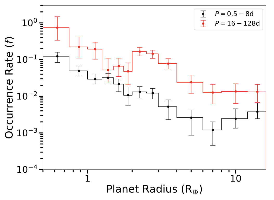
Fig. 1.6 The occurrence rate of planets across a wide range of planetary radii and over two period ranges (short period, black; long(er) period, red). Note that neither of these period ranges include the orbital period of Earth. The broad patten is of significantly higher planet occurrence rates for smaller planets. This estimate is for FGK-type stars. From Hsu+2019.

C1 ‘The origins of planets’ will go into more detail on many of the topics on planet discovery covered here.

\(n_e\), the number of planets per star capable of hosting life

Now we begin to leave the realm of the known. The fundamental challenge with estimating the number of planets per star capable of hosting life, as with many of those parameters remaining, is that it requires us to know something general about life as a phenomenon. Achieving this seems far off, given we are unable to agree on a definition of life, and even whether a definition is useful, e.g., Szostak, 2012.

The problem becomes more tractable if we think about Earth-like life, C-H-N-O-P-S-based and requiring liquid water. In this case, it is the water phase diagram that places the tightest constraints on life’s preferred pressure/temperature range. With water available in its biologically-essential liquid form over a relatively narrow window at Earth’s surface pressure. In this framework we are looking for the occurrence rate of planets in the liquid-water habitable zone around stars, which is something we might be able to estimate (see above, the fraction of stars hosting planets) and Fig. 1.7).

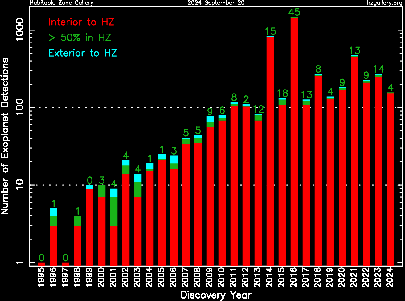
Fig. 1.7 Habitable zone planet discoveries through time. Note, in many cases these are massive planets. Credit: Habitable Zone Gallery.

The number of planets per star capable of hosting life is a parameter that crosses content in C1 ‘The origins of planets’, with planet formation clearly being critical for whether a habitable planet emerges, and also C2 ‘The origins of habitable environments’, where the processes underpinning planetary habitability are looked at in more detail. In principle, as the ability to host life is predicated on the life itself, this really is a parameter that reaches into content in C3 and C4 as well.

\(f_l\), the fraction of habitable planets developing life

To move onto this parameter we need to carry a definition of habitability with us, and so an implicit assumption of the chemical physical conditions life requires. For practical purposes, we will continue in the liquid-water habitable zone paradigm. Although this is something you might want to question.

The frequency of habitable planets that go on to develop life is a fascinating question, one that reaches to the heart of whether the emergence of life on Earth is a one-off or an inevitability given clement conditions at a planet’s surface. Standing where we are, not having a complete origin of life scenario (seeming in fact far from it), life’s emergence appears fantastically complex and unlikely. However, once the chemistry is worked out, maybe we will view it more as chemical necessity.

Lacking a chemically complete origin of life scenario, there are two observational fronts on which we could in principle make progress with the question of the frequency of inhabited planets:

1. Solar system exploration: The most immediate prospect for discovering whether there was an independent origin of life scenario in the solar system is our exploration of Mars. Recent observations have found curious features on the surface of martian rocks (see Fig. 1.8; Hurowitz+2025), which would superficially be consistent with microbial activity. Ultimately, only sample return to Earth will be able to resolve this question. However, we now have abundant evidence that Mars had at least transient wet periods in its history (e.g., see C2, and Wordsworth+2021).

2. Biosignature searches on exoplanets: trace atmospheric constituents may indicate the presence of life, such as ozone on Earth. These are rarely on their own unambiguous evidence of life, and context is essential: the phosphine molecule, which on Venus led to the suggestion of life being present to produce it (Greaves+2021), on Jupiter is a stable constituent of the atmosphere, with no life required (Prinn & Lewis 1975). If with present or future observatories a biosignature anomaly is persistently associated with habitable zone planets, it may be enough to convince the community that life is present and frequently occurring on suitable planets.

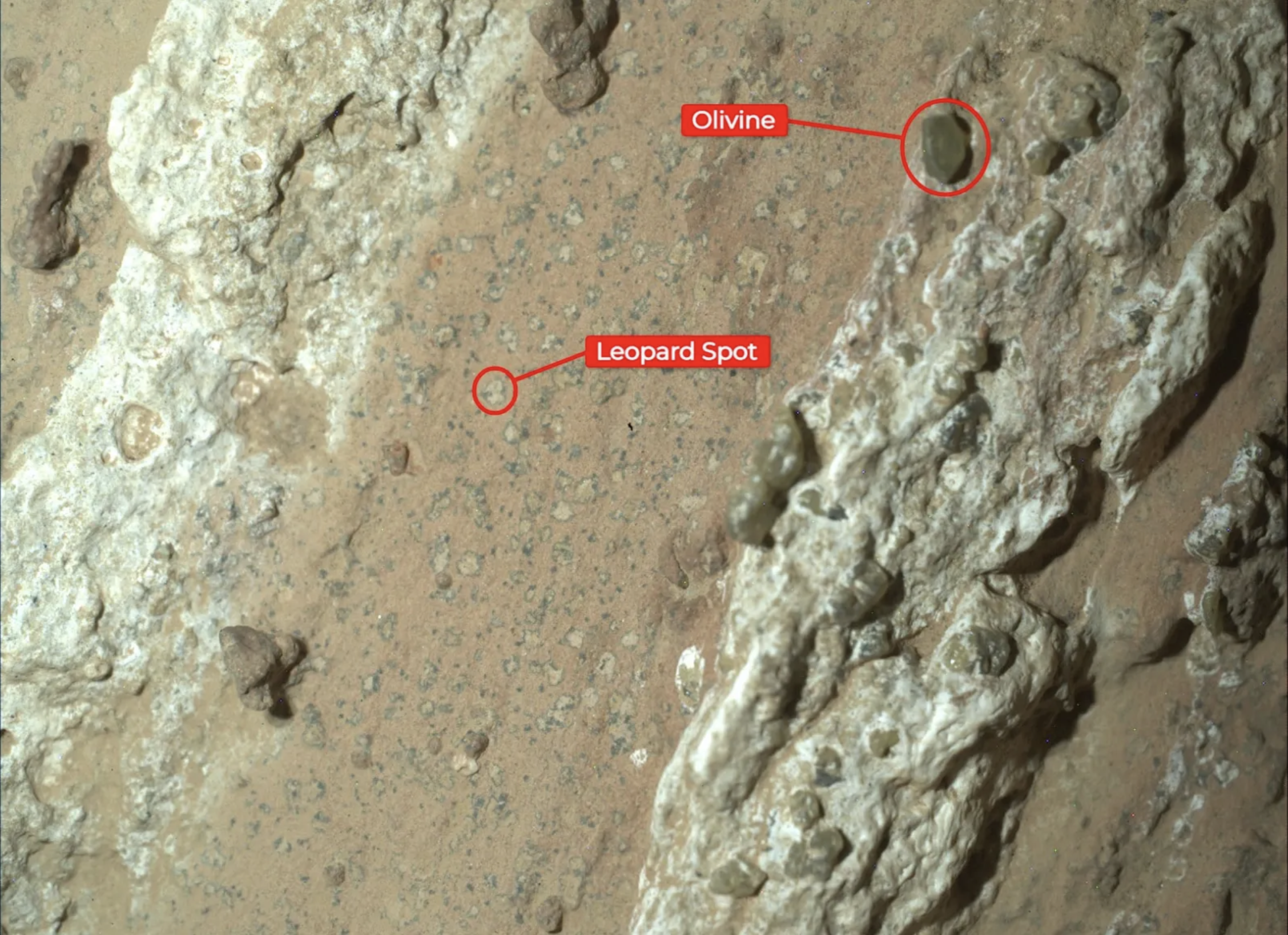
Fig. 1.8 Leopard spots on a martian rock. Signs of life? Image: NASA/ JPL-Caltech/ MSSS.

The frequency of habitable planets that go on to develop life is a parameter that could be thought about through Core Course material in C2 (where we consider the geological history and exploration of Mars), C3 (where we think about detecting life), and C4 (where we consider the history of life on Earth).

\(f_i\) and \(f_c\), the fraction of biospheres that develop ‘intelligence’ and communication

These two parameters take us now far beyond what even hypothetical and outstanding discoveries in the solar system, such as evidence of ancient life on Mars, could tell us about. The only prospect for having informed insight into these numbers is for the SETI programme to be successful.

\(L\), the mean communication timescale

The mean communicative timescale for a civilisation is also unknown a priori. However, our own history is interesting in this regard. Radio broadcasts began only just over a century ago, but we are already moving away from using isotropically emitted radio frequency broadcasts to focussed communication, using satellite and fibre optic connections. If the kind of radio signals that propagate isotropically into the galaxy are only a short-lived technological stage, then this mean timescale may be very short, and the chance of finding technological life by this means correspondingly small.

How relevant is the Drake equation?

Given the previous sections, it is clear we are not in a position to fully evaluate the Drake equation and obtain a value of \(N_c\), the mean number of communicative civilisations in the galaxy, without significant, and essentially completely unconstrained, assumptions. However, we work with numbers like \(N_c\) frequently as scientists, it is just the Drake equation asks too general a question we cannot fully resolve. For example, if instead we ask ‘how large a volume of space (centred on Earth) do we need to survey to find 10 hot Jupiters?’, then we are asking a question much like the Drake equation, but now one that is fully tractable given present information. What is more, this question, and ones like it, are exactly the types of questions you would ask if you were proposing an observing campaign: it is critical to know that the observing resource you request will deliver the science result.

So, it is not that the type of question is wrong, just that the amount of information required to answer it in this form makes it intractable. Just by removing a couple of terms from the Drake equation (1.1), it becomes more relevant to a general search for life in the Universe – we might settle in the first instance for the life we are searching for not being ‘intelligent’, giving

(1.2)\[N_l = R_* \cdot f_p \cdot n_e \cdot f_l \cdot L_s.\]

Here, we have dropped the most problematic terms from (1.1): the propensity for life to become ‘intelligent’ and communicative. We are then left with an expression evaluating to give \(N_l\), the mean number of life-hosting planets in the galaxy, and instead asking that we now know \(L_s\), the mean longevity of life on a planet.

The term that is most unknown in this expression is \(f_l\). However, the final term has now become something that we might venture more of an opinion on than the mean communicative timescale, \(L\).

Life on Earth has shown remarkable resilience since its emergence > 3.5 Ga, surviving near global glaciations, major asteroid impacts, and numerous large outpourings of magma. Over this period, life has also been hugely diverse, evolving from single cell, to multicellular, to the macrobiota that covers most of Earth’s continents today. All these types of life have proven resilient to large perturbations of their environments, even as species have gone extinct. More on this in the Core Course’s final module.

Life on Earth suggests that once established, and provided the planetary climate remains within habitable bounds somewhere on its surface, life will survive in refugia, radiating outwards when conditions allow. Having a sense of values for \(R_*\), \(f_p\), and \(n_e\) from astronomical observations, \(f_l\) stands out as the parameter with most potential to cause \(N_l\) to evaluate to a small number.

How would you re-write the Drake equation and evaluate it for the search for life in the Universe?