2.10. Planet formation II: Differentiation

Professor: Oliver Shorttle (IoA, Department of Earth Sciences)

---

Learning objectives:

• Identify the drivers of differentiation

• The physical-chemical basis for differentiation

• The chemical consequences of differentiation

• The use of partition coefficients for determining core/mantle composition.

• The origin and use of oxygen fugacity as a concept

• Understand the meaning and significance of oxygen fugacity as an intensive thermodynamic property of planetary systems

• Differentiation in the context of planetary crusts and atmospheres

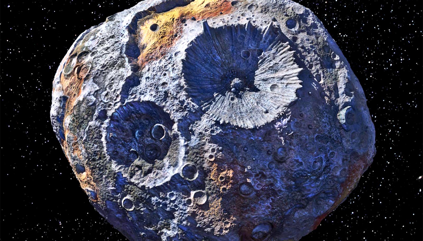
Fig. 2.59 The asteroid 16 Psyche is the focus of the NASA Pysche mission. It is being targeted because it is metal rich, possibly being the remnant core of a once larger planetesimal. Image credit: Maxar/ASU; P. Rubin/NASA/JPL-Caltech.

In this lecture we look at the processes that take the building blocks of planets and create something new, a planet segregated into compositionally distinct layers. This is a process with important consequences for the habitability of the surface environment, as gasses are released to the atmosphere, the crustal substrate of life is created, and metals are permanently sequestered to the planet’s core.

What is differentiation?

The gravitationally driven chemical segregation of material in a planet.

Essential to differentiation is that chemical differences between phases in a body can be operated on by a gravitational field to produce large scale separation.

Some of the key processes occurring during differentiation are illustrated in Fig. 2.60, focussing on how the life-essential elements CHNOPS are affected. From bottom right clockwise around the figure this schematic tracks progressive heating of the growing body, through metamorphism (Fig. 2.60-1), melting (Fig. 2.60-2), metal segregation and core formation (Fig. 2.60-3), and finally magma ocean solidification (Fig. 2.60-4), which precipitates the beginning of secondary differentiation forming crusts and atmospheres.

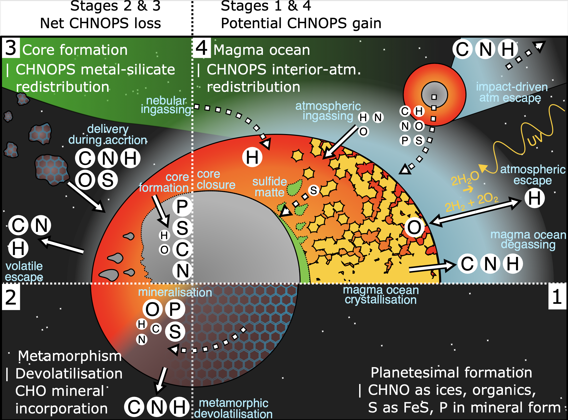
Fig. 2.60 An illustration of processes occurring during an object evolving from an undifferentiated asteroid/planetesimal through to a fully differentiated body. The stages shown are: (1) planetesimal assembly, (2) planetesimal heating by short lived radionuclides decay driving metamorphic volatile processing and loss, (3) eventual planetesimal melting and growth, and (4) and magma ocean crystallisation. During this period the object is still growing as accretion proceeds. Image from Krijt+2022.

What drives differentiation?

As emphasised above, differentiation is possible because of the inhomogeneity of phases in a planet. We can see this inhomogeneity beautifully in chondrites, the undifferentiated precursors to planets. These contain separate metal, crystalline silicate, and amorphous phases, each with different physical properties, and critically, densities. Of these metal is most dense, and provided it does not become oxidised during heating, will sink in a mixed silicate-metal melt.

Why is there metal?

The presence of dense metal alloys in the building blocks of planets is key to their first major phase of differentiation, and also of course drives their subsequent magnetic fields. But why is their sufficient metal to segregate as a discrete phase?

At Earth’s surface we are used to metals rapidly oxidising. However, at a planetary scale the amount of metals competing for oxygen far exceed the amount of oxygen present in the planet. All the major elemental constituents of Earth’s mantle form oxides: \(\mathrm{SiO_2}\), \(\mathrm{Al_2O_3}\), MgO, and CaO. Iron has the least affinity for oxygen of all these metals, with the result that it is what is left over once all the oxygen has been used up.

The cause for excess Fe is evident from Fig. 2.61: there is a peak in its abundance prior to the rapid decline in abundance of heavier elements. This results from iron’s nuclear stability, so that neutron addition reactions inside stars terminate at Fe, after which further neutron addition builds less stable rather than more stable nucleii. The fate of planets to differentiate to have metal cores is therefore written in the nucelear physics of the Universe.

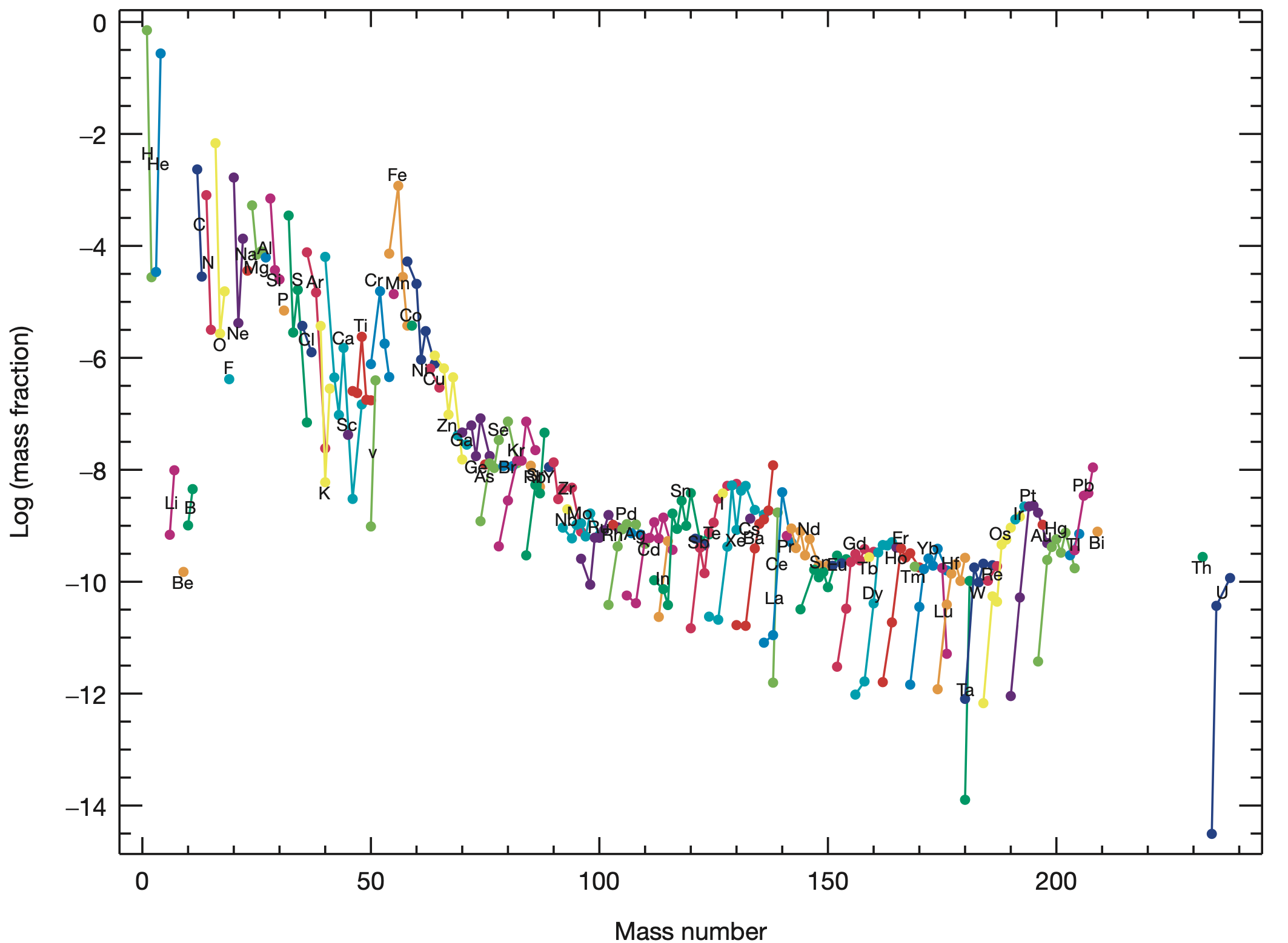
Fig. 2.61 The major differentiation episode planets experience is driven by segregation of (dominantly) Fe-metal to form their core. This is possible because of the nuclear stability of iron, resulting in its accumulation during nucleosynthesis and comparatively high abundance for an element of its atomic mass. This is visible in the figure here, plotting the abundance by mass of isotopes present in solar system matter according to their atomic mass. From Heger+2014.

What is oxygen fugacity and how is it useful?

We talked above about the fact that the iron that is present in primitive meteorites will sink and form cores if it is not oxidised. This brings us to the concept of oxygen fugacity…

Oxygen fugacity is a concept that will come up frequently when planetary interiors are discussed, often in relation to how they might interact with their atmospheres. It is just a measure of how oxidising a system is, expressed in terms of the fugacity of \(\mathrm{O_2}\) gas that the system is (or would be) in equilibrium with. The ‘fugacity’ part of this is just talking about the effective partial pressure of the oxygen gas, ‘effective’ because intermolecular interactions might cause the partial pressure to be different compared to if those interactions did not take place.

If we stick to thinking about oxygen fugacity in low pressure systems, then partial pressure and fugacity are roughly equal. The oxygen fugacity of Earth’s 1 bar atmosphere, with ~21% oxygen, is just 0.21 bar.

What the above means is that a system with a higher oxygen fugacity, or \(f_\mathrm{O_2}\), is more oxidising than a system with a lower \(f_\mathrm{O_2}\). Conceptually, this would mean if you could put the two systems next to each other separated by a membrane that only allowed oxygen to pass across it, oxygen would flow from the oxidising to the reducing system. The more oxidising system might have more \(\mathrm{CO_2}\) than CO, more \(\mathrm{H_2O}\) than \(\mathrm{H_2}\), and more FeO than \(\mathrm{Fe^{metal}}\).

Often, \(f_\mathrm{O_2}\) is written out not as its raw fugacity but as \(\log_{10}(f_\mathrm{O_2})\), because the numbers involved are so small. Somewhat confusingly, geologists often report how oxidising a system is by comparing the \(f_\mathrm{O_2}\) to that of another system altogether. The logic for this is that a lot of ‘trivial’ variation in \(f_\mathrm{O_2}\) is driven by variation in temperature and pressure, which we want to see through to how oxidising a system intrinsically is (see Fig. 2.62). comparing it to another system with similar pressure and temperature dependence of its \(f_\mathrm{O_2}\) can be useful. Such relative oxygen fugacities are often expressed as \(\Delta \text{reference system}\), e.g., \(\Delta \mathrm{IW}\) where the reference system is the equilibria between iron metal and iron oxide, which we look at below.

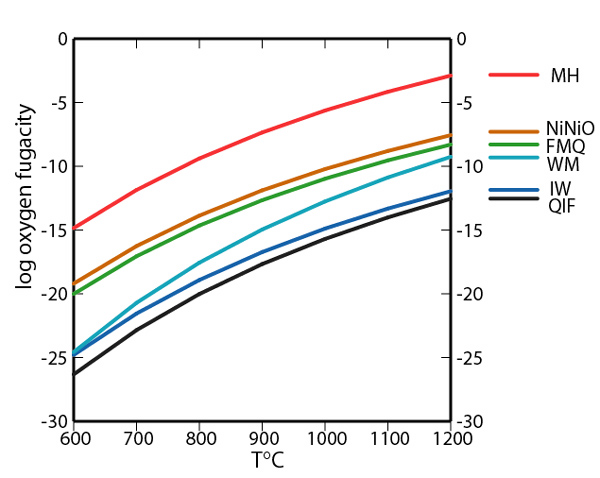
Fig. 2.62 The temperature dependence of common reference redox equilibria (‘buffers’) discussed in the Earth Sciences. The y axis is \(\log_{10}\) of the fugacity of oxygen in bar. The strong temperature dependence is evident: all equilibria become more oxidising as temperature increases, and nearly all do so at the same rate - hence the ability to compare to one of these equilibria and control for ‘trivial’ effects of temperature. The acronyms are based on the first letters of the phases involved in the equilibria, ordered here from most oxidising equilibria to most reducing: MH = magnetite hematite \(\mathrm{2Fe_3O_4 + 1/2O_2= 3Fe_2O_3}\); NiNiO = nickel nickel oxide, \(\mathrm{Ni + 1/2O_2 = NiO}\); FMQ = fayalite magnetite quartz, \(\mathrm{3Fe_2SiO_4 + O_2 = 2Fe_3O_4 + 3SiO_2}\); WM = wustite magnetite, \(\mathrm{3FeO 1/2O_2= Fe_3O_4}\); IW = iron wustite, \(\mathrm{Fe + 1/2O_2 = FeO}\); QIF = quartz iron fayalite \(\mathrm{SiO_2 + 2Fe + O_2 = Fe_2SiO_4}\)

It is useful to see how oxygen fugacity is related to chemical equilibria. The relevant example we will explore for this lecture is the chemical equilibria between iron metal (Fe) and iron oxide (FeO):

(2.10)\[\mathrm{Fe^{0} + 1/2O_2 = Fe^{2+}O}.\]

We will now rewrite this equation to show how the \(f_\mathrm{O_2}\) of a planet is a measure of how much iron is left in its mantle after core formation.

Equation (2.10) captures the fact that the equilibrium between these two iron-containing phases must also involve a free oxygen phase, even if it is present in vanishingly small quantities. It is important to understand that neither the FeO nor the Fe need to be a pure phases, for example the FeO could be dissolved in a silicate liquid (a magma) and the Fe metal could be part of a metal alloy (e.g., with Ni).

To bring oxygen fugacity into this equation, we need to write out the equilibrium constant

(2.11)\[K_{eq}(T,p) = \frac{\mathrm{a_{FeO}}}{\mathrm{a_{Fe}}f_\mathrm{{O_2}}^{1/2}},\]

where \(a\) denotes activity of the corresponding component, and \(f_{O_2}\) is the fugacity of oxygen – numerically equivalent to activity when we choose our units as bar and reference pressure as 1 bar.

We can also usefully rewrite the activity terms to include things we can measure (concentrations) and things we can experimentally determine (how the concentrations map through to activity), giving

(2.12)\[a_i = x_i \cdot \gamma_i,\]

where \(x_i\) is the mole fraction of component \(i\), and \(\gamma_i\) is the rational activity coefficient, introduced to account for non-ideal behaviour of components (equivalent to the relationship between partial pressure and fugacity for gasses). If we proceed by assuming these non ideal terms are not important (i.e., are close to unity), we obtain

(2.13)\[f\mathrm{_{O_2}} = \left(\frac{x_\mathrm{FeO}}{x_\mathrm{Fe}K(p,T)}\right).\]

By further assuming that the metal is pure Fe, we obtain a simple expression where now how oxidising the system is just depends on the equilibrium constant and the FeO concentration of the silicate.

(2.14)\[f_\mathrm{O_2} \sim \left(\frac{x_\mathrm{FeO}}{K(p,T)}\right)^2.\]

From equation (2.14), and coming back to the question of planetary differentiation, we see that more oxidising planets have more FeO in their mantles. In this sense then Mars, with ~17% by weight FeO in its mantle is globally more oxidising than Earth, with 7% by weight in its mantle and a much larger core.

…However, things are never quite so simple with the oxygen fugacity of planetary interiors. While bulk Mars is globally more oxidised than Earth, Earth’s mantle in isolation is more oxidising than that of Mars. This because a second process, subject to much debate (e.g., read more in Frost+2008), has taken some of the FeO in Earth’s mantle and produced \(\mathrm{Fe_2O_3}\), oxidising the iron and thereby Earth’s mantle slightly above what would be expected from simple core–mantle (metal–silicate) equilibration.

Heat and differentiation

The formation of cores both requires heat and liberates heat. Core formation requires heat as without it bodies remain isotropic, with their chemical inhomogeneities distributed throughout and unable to segregate. Sufficient heat drives melting of a planetesimal and allows gravity and fluid dynamics to act to bring dense material to the centre of the planet. There are two main sources of heating that we discuss here.

Heat from accretion

The first source of heat to growing planets is from accretion itself. The maximum available energy for heating is from the conversion of gravitational potential energy to kinetic energy and then eventually heat as material falling into the gravitational potential well of the planet reaches its surface. The equation for this energy is

(2.15)\[U = -\frac{3}{5}\frac{GM^2}{R},\]

where \(G\) is the gravitational constant, \(M\) is the mass the planet grows to, and \(R\) is the radius is grows to.

Taking equation (2.15), the results are plotted in Fig. 2.63 across of range of planetary radii. Solar system planets are also plotted for reference.

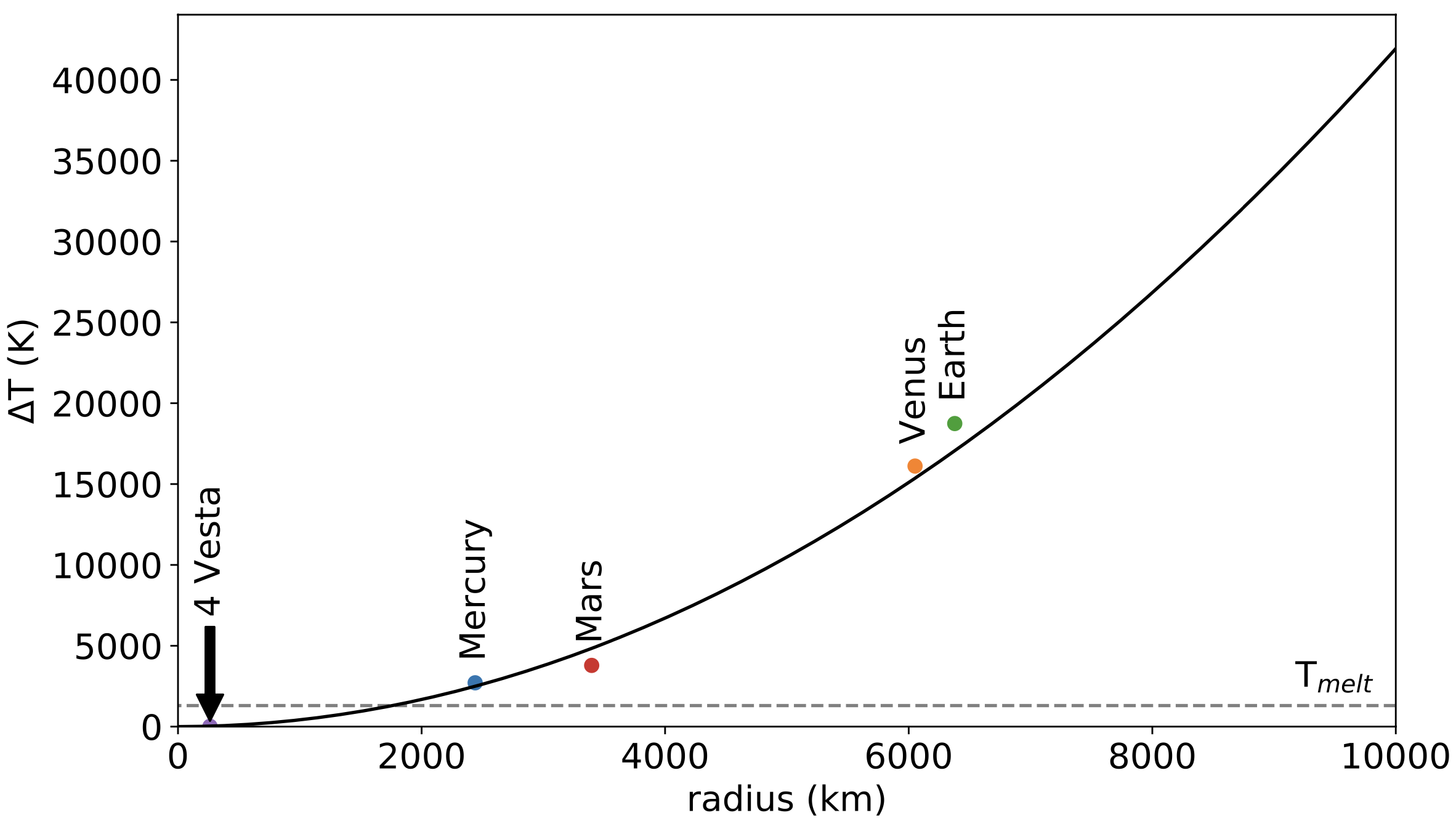
Fig. 2.63 The temperature that accretion alone will heat bodies to as a function of their size. Assuming no heat loss during accretion. Solar system planets are plotted for reference, and fall off of the line because their observed masses and radii are used, rather than assuming a fixed M-R relationship as in the black line.

An important observation from Fig. 2.63 is that if we assume melting should not take place until \(\Delta T =1500\,\mathrm{K}\), then only bodies exceeding 1500 km should melt. This is nearly the size of Mercury. However, we see much smaller differentiated objects in the solar system, a prominent example being 4 Vesta, which has a radius of 262.7 km.

There must be another source of heat to young planets to drive their differentiation.

Heat from radionuclide decay

The second key source of heat to young planets is radioactive decay. The decay of radionuclides provides an important source of heat on Earth today, however, this was even more important early in the solar system’s history, when short lived radionuclides, those that decay rapidly and are today extinct, were still abundant. We look at a simple calculation for this heat source here.

The rate of decay of radionuclides is given by

(2.16)\[\frac{dN}{dt} = -\lambda N(t),\]

where \(N(t)\) is the number of nuclides of a given radioisotope remaining at time \(t\), and \(\lambda\) is the decay constant (\(\mathrm{s^-1}\)).

The key short lived radionuclide that drove a lot of heating in the early solar system was \(\mathrm{^{26}Al}\). It decay scheme is

(2.17)\[\mathrm{^{26}Al \rightarrow ^{26}Mg^* + (\epsilon, \beta^+) \rightarrow ^{26}Mg + \gamma}.\]

\(\mathrm{^{26}Al}\) first decays to an excited state of \(\mathrm{^{26}Mg}\), emitting a positron and neutrino, the excited nucleus then decays to ground state by emitting a gamma ray (\(\gamma\)). This is shown in Fig. 2.64.

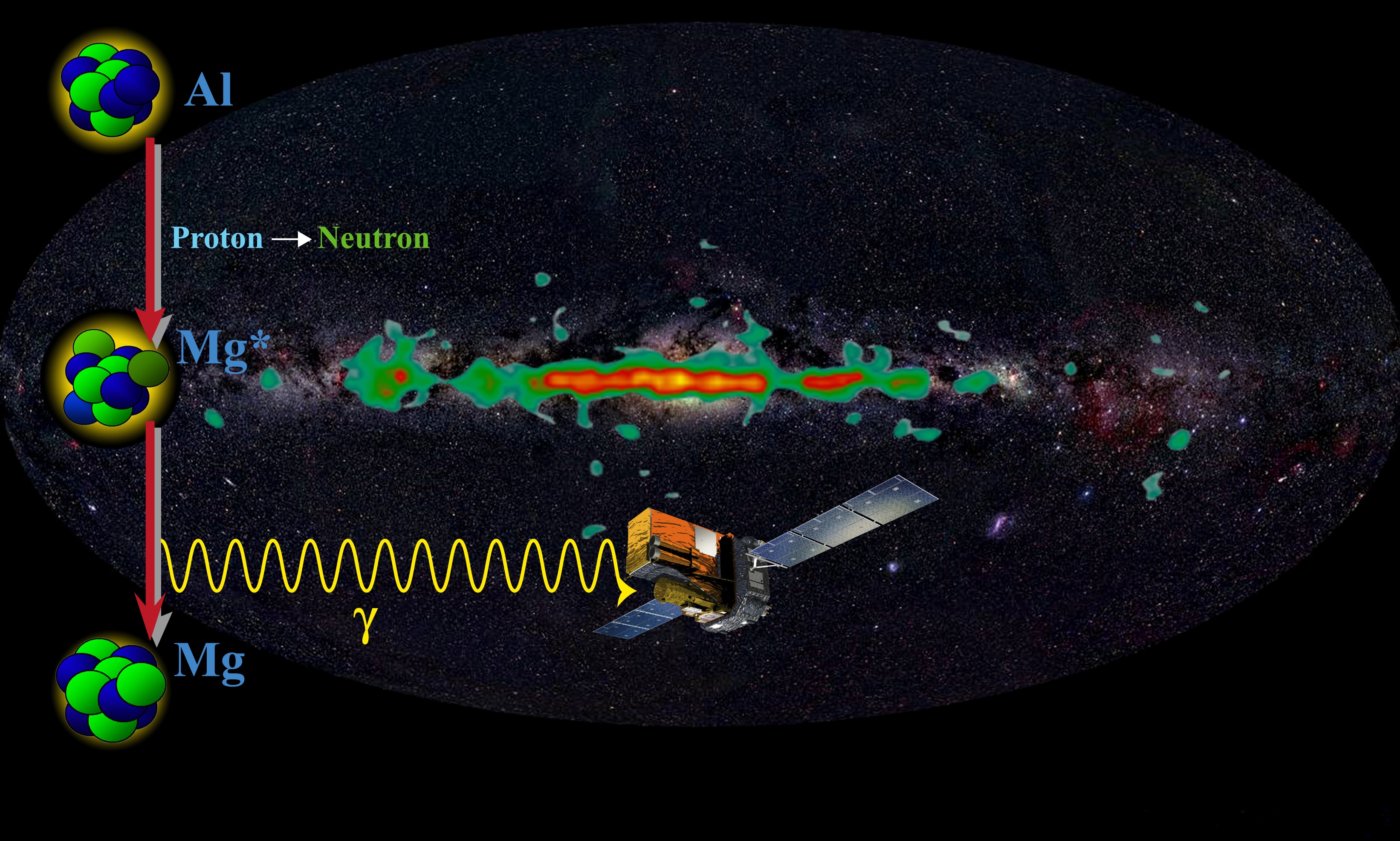
Fig. 2.64 A schematic of the decay sequence of \(\mathrm{^{26}Al}\) and a map of its associated gamma ray emission throughout the galaxy. Emission is notably concentrated towards the galactic midplane and peaks towards the galactic centre, both regions where star formation rates are higher. Image credit: R. Diehl, MPE, Germany.

We can relate the rate of temperature change to the rate of heating and the heat capacity of the body,

(2.18)\[\frac{d\Delta T}{dt} = \frac{Q(t)}{C_p},\]

where \(Q(t)\) is the heating rate per unit mass (\(\mathrm{W\,kg^{-1}}\)) and \(C_p\) is the isobaric heat capacity (\(\mathrm{J\,Kg^{-1}\,K^{-1}}\)).

The heating rate is given by

(2.19)\[Q(t) = Q_0x_0\exp(-t\ln 2 / t_{1/2}),\]

where \(Q_0\) is the heating rate (\(\mathrm{W\,kg^{-1}}\)) from a given radionuclide at \(t=0\), \(x_0\) is the concentration by mass (i.e., \(\mathrm{kg\,kg^{-1}}\)) of that radionuclide at \(t=0\), and \(t_{1/2}\) is the halflife of the radionuclide (\(\mathrm{s}\)).

If we combine equations (2.18) and (2.19) and integrate then we obtain the change in temperature driven by radionuclide decay, assuming no heat lost. Using appropriate numbers (0.355 W/kg for \(\mathrm{^{26}Al}\) heating and an estimate of its initial abundance of \(\mathrm{5\times10^{-5}}\) atoms of \(\mathrm{^{26}Al}\) per \(\mathrm{^{27}Al}\) atom) into the resulting equation shows that heating from radionuclide decay can readily melt the entire body.

Chemistry of differentiation

Differentiation represents a major episode of elemental redistribution in planets. We can see its effect in the composition of the bulk silicate Earth, shown in Fig. 2.65, which records major depletions in siderophile elements, those elements with an affinity for metal.

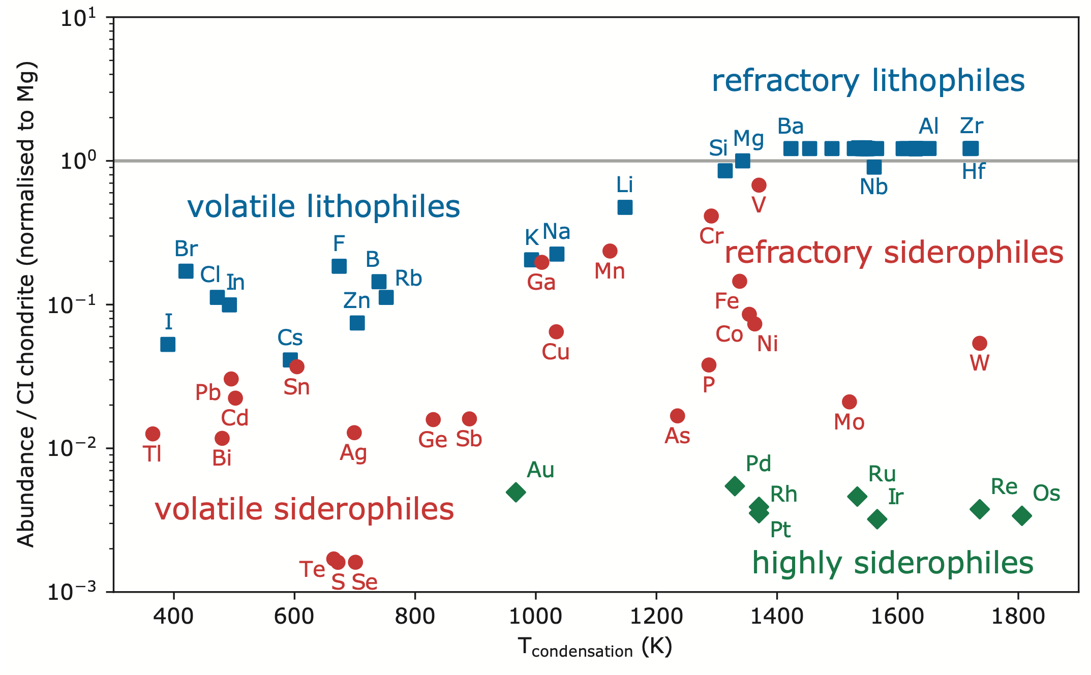
Fig. 2.65 The fingerprint of core formation in the Earth. The abundance of elements in the Earth’s mantle normalised to the element’s abundance of the element in the sun (with secondary normalisation to Mg to account for Earth’s lack of \(\mathrm{H_2}\), as a function of the half mass condensation temperature of the element. Elements with an affinity for metal, siderophile elements, are strongly depleted. From Guimond+ 2024.

The distribution of siderophile elements between silicate and metal, when equilibrated, can be described using partition coefficients, calculated as

(2.20)\[D_i^{1,2} = \frac{x^1_i}{x^2_i},\]

where \(D_i^{1,2}\) is the partition coefficient for element \(i\) between phases \({1}\) and \({2}\), and \(x\) represents the concentration of this element in each phase. Partition coefficients are a function of pressure, temperature and oxygen fugacity, and ultimately need to be constrained on an element by element basis experimentally. However, they offer a powerful means of predicting the composition of planetary mantles left after core formation, and for an observed mantle, use the sensitivity of the partition coefficients on intensive thermodynamic variables to reconstruct the conditions of core formation.

A summary of how elements across the periodic table are classified according to their affinity for certain states of matter is given in Fig. 2.66.

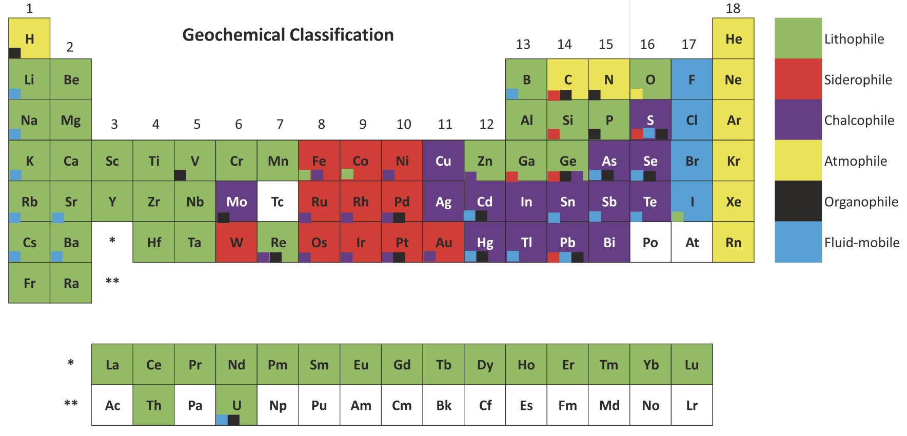
Fig. 2.66 A representation of the periodic table emphasising how the chemical behaviours of the elements affect their fate during planetary differentiation. Image from Lee, 2016.

Secondary differentiation

Secondary differentiation is the term we are using here to refer to all the planetary differentiation that occurs after core formation. Most importantly, this produces crusts and atmospheres.

Crusts

The formation of crusts on planets, as chemically distinct reservoirs to their mantles, is a result of how melting of rocks (and indeed any multi-component system) operates. While we are used to the melting of water from daily life, where solid water (ice) goes to liquid water without any (discernable) change in composition (a one component system of \(\mathrm{H_2O}\)). This is generally not the case for more complex systems.

We illustrate this point in Fig. 2.67. This is showing the melting of a Cu-Ni alloy as temperature rises. Critically, as temperature is increased, melting does not just happen at a single temperature, as it would do for pure water ice, but across a range of temperatures. Across this temperature interval the liquid produced is a different composition to the solid it leaves behind. This is called partial melting, and is the reason that melt production on planets produces chemically distinct crusts.

While Fig. 2.67 represents

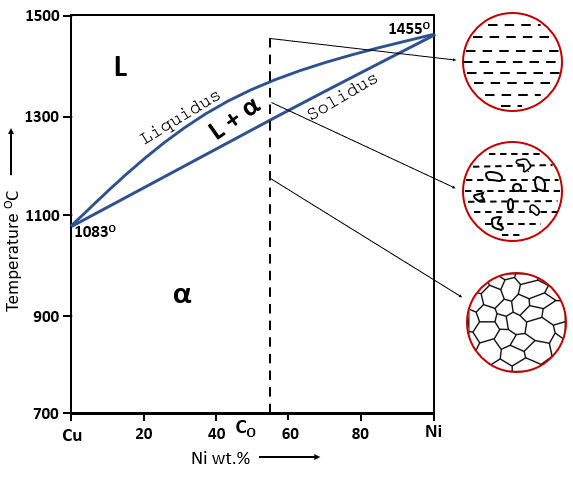
Fig. 2.67 A phase diagram for a Cu-Ni alloy – the horizontal axis describes the composition of the phases present. In the lower temperature region, phase \(\alpha\), Cu and Ni are fully miscible and form a single phase. In the upper high-temperature region, phase ‘L’, the system is a fully molten liquid. The middle region, at intermediate temperatures and bracketed by a ‘liquidus’ and a ‘solidus’ surface, is the region where solid and liquid coexist. In this region, the system splits into two phases of different composition to each other and to the system’s bulk composition (which by necessity remains unchanged). Physical segregation of liquid from solid then creates two compositionally new domains. Image credit: LearnMetallurgy.

Although Fig. 2.67 represents a very simplified version of partial melting, this is the thermodynamic essence of what happens in Earth’s mantle. It is also what happens when you melt the crust itself, which must have occurred to turn what would have originally been a basaltic composition crust (the composition of melt obtained from melting the mantle) into the andesitic continental crust we live on.

The effect of this successive differentiation through partial melting on the composition of Earth’s rock reservoirs can be seen from Table 2.2.

Table 2.2 The major element composition of Earth’s crusts compared to its mantle. All compositions in weight percent (not renormalised to 100%). Compositions from McDonough & Sun (1995) (mantle), Workman & Hart (2005) (basalt), and Rudnick & Gao (continental crust).

	\(\mathrm{SiO_2}\)	\(\mathrm{Al_2O_3}\)	\(\mathrm{FeO}\)	\(\mathrm{MgO}\)	\(\mathrm{CaO}\)	\(\mathrm{Na_2O}\)
Mantle (peridotite)	45.0	4.5	8.1	37.8	3.6	0.4
Oceanic crust (basalt)	49.5	16.8	8.1	9.7	12.5	2.2
Continental crust (andesite)	60.6	15.9	6.7	4.7	6.4	3.1

The emergence of Earth’s continental crust, how and when, has been a long running point of debate in the Earth Sciences. The level of disagreement about when is captured in Fig. 2.68, which shows the range of trajectories for the growth of Earth’s continental crust researchers have proposed. All growth curves in Fig. 2.68 delay the onset of significant continental crust production until millions of years after Earth’s formation, recognising that this differentiation process needs to act on top of the earlier formation of basaltic crusts.

The use of partition coefficients ((2.20)) can also be used to understand compositional changes associated with crust formation. In this application, the two phases of interest are silicate melt and the residual solid silicate, rather than the silicate and metal we were considering for core formation

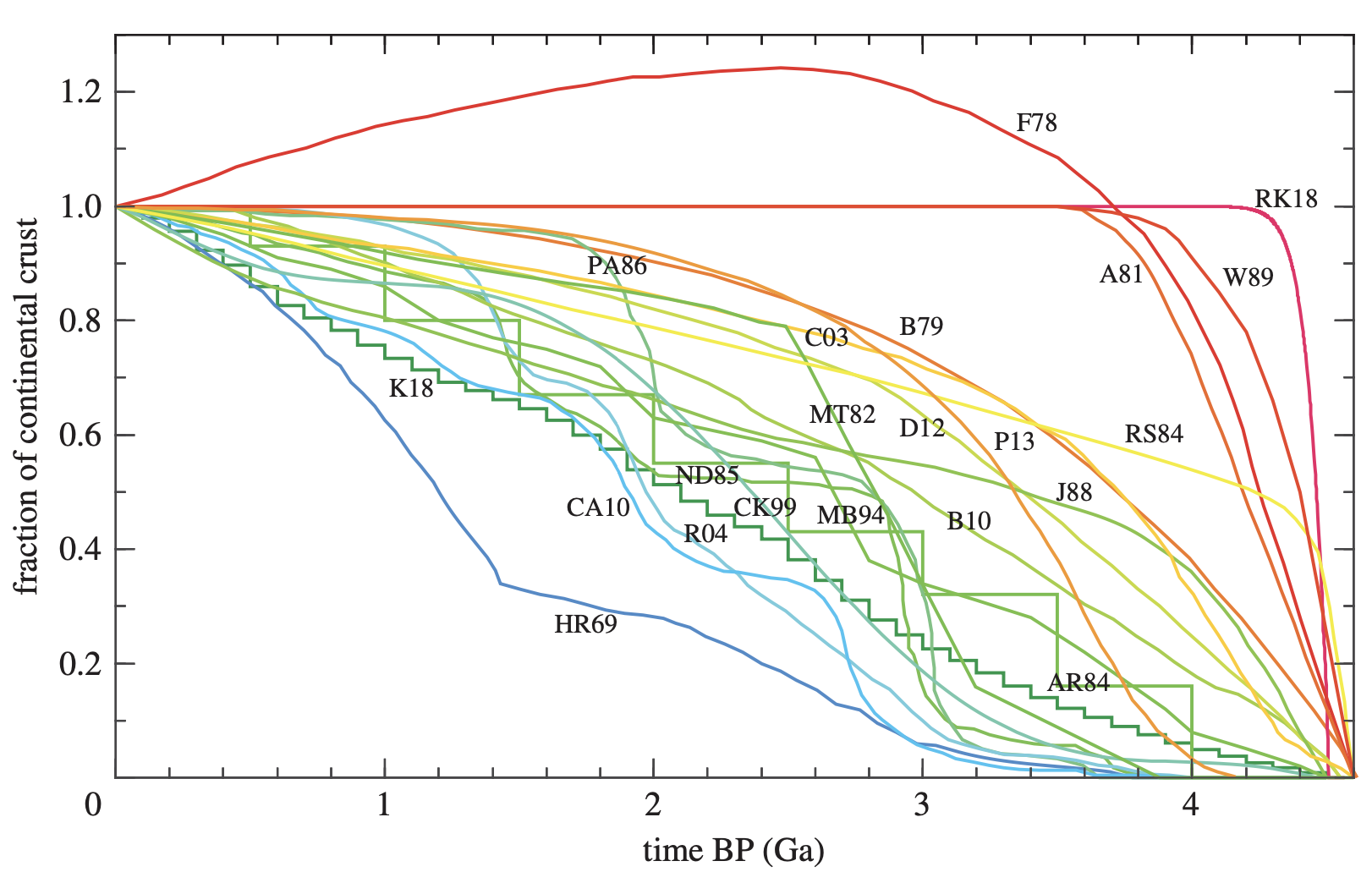
Fig. 2.68 A classic way to look at the evolution of Earth’s continental crust is to plot the fraction that existed (typically a mass fraction normalised to its present mass, as here) as a function of time. Clearly there is wild disagreement about when the substrate for most life on Earth arose. Some models even posit a higher continental crustal mass in the past compared with today. From Korenaga, 2018.

Earth is unique in the solar system in having an extensive crust of more silica-rich composition (Table 2.2). This perhaps touches on the why of Earth’s crust formation, and that it is linked to its unique regime of plate tectonics.

Atmospheres

Atmosphere formation produces the outer shell on a planet. In many respects this is simply another form of differentiation, taking volatile or atmophile elements (Fig. 2.66) and moving them to the surface of a planet.

Formation of atmospheres from the material initially contained in planetary interiors is driven by volcanism. The formation of a magma by partial melting in a planet’s mantle moves elements like carbon and hydrogen from the solid silicate into the melt (these elements have low solid-liquid partition coefficients, (2.20)). When the magma reaches low pressure, these gases begin to exsolve from the melt, just like carbon dioxide leaving a fizzy drink when you release the cap. Different gases have different solubilities in the magma, leading to gases of different composition depending on the pressure at which degassing occurs (Fig. 2.69).

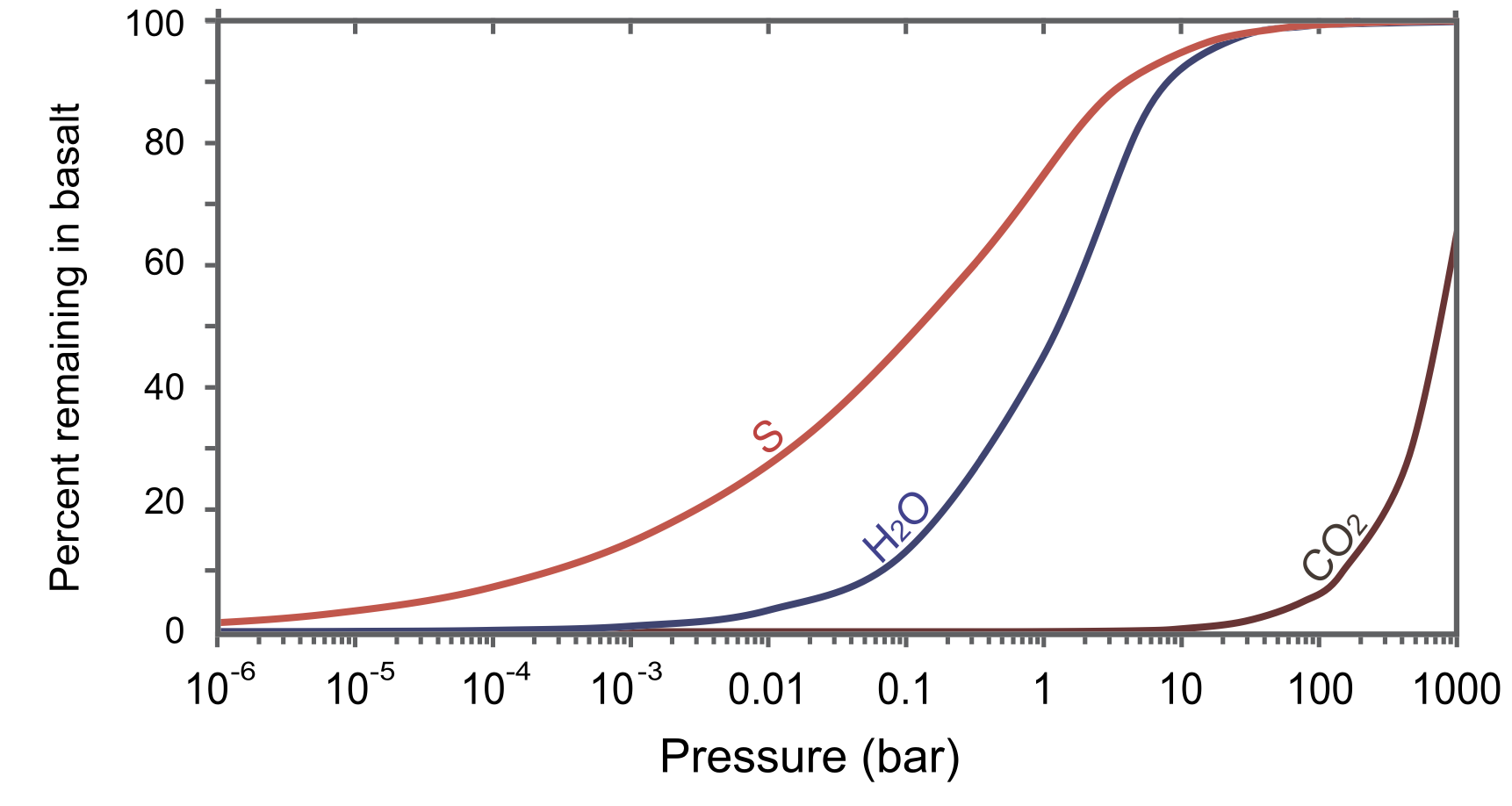
Fig. 2.69 . Modified from Gaillard, 2014.

Another key parameter describing gas chemistry is oxygen fugacity. Changes in \(f\mathrm{O_2}\) affect the relative proportions of, for example, \(\mathrm{CO_2}\) to CO and \(\mathrm{H_2O}\) to \(\mathrm{H_2}\). See Gaillard+2014 and Gaillard+2021 for more discussion of this.