4.7. Atmospheric Chemistry II

Professor: Alex Archibald (Yusuf Hamied Department of Chemistry)

---

Photochemistry

The energy from the nearest star can be a key driver for the chemistry of planetary atmospheres in a solar system. Assuming that the star can be represented as a blackbody emitter, Wiens displacement law (\(\lambda_{\rm max} = b/T\)) can be used to predict the peak wavelength of solar radiation reaching the top of the atmosphere (TOA). As this radiation travels through the atmosphere it is either absorbed or transmitted or reflected.

Molecules poses a finite number of energy levels, with the spacing between these determined by the structure and composition of the molecules/atoms. When a photon is absorbed by a molecule a number of processes occur. Essentially we are delivering energy to the molecule so the molecules increase their “energy level” with a range of consequences.

Fig. 4.59 The photo processes possible for CH\(_3\)CHO under irradiation of UV light. After Rowell et al., 2022

Fig. 4.59 shows the processes that can occur following the absorption of a photon of light (hv) for the simple organic molecule acetaldehyde (CH\(_3\)CHO). On the left hand axis we see energy and on the right hand axis the photon wavelength and we see that photons with wavelengths of less than 350 nm have enough energy to go from the ground electronic state (S0) to the first excited electronic state (S1). The diagram shows us that in this case, the excited state is still a bound state – we have excited our molecule but not photo-dissociated it. However, through a process called inter system crossing (ISC) other states are accessible which can lead to rearrangement (o form the keto-enol form CH\(_2\)CHOH) and dissociation.

Calculation of photolysis rate coefficients

Atmospheric chemists commonly use the symbol \(k\) for a reaction rate coefficient that involves molecular “collisions” and the symbol \(J\) for a reaction rate coefficient for a reaction that involves the absorption of photons resulting in molecular dissociation. We call this process photolysis (photo-dissociation or photodecomposition). The rate coefficient of photolysis of a constituent, \(i\), (\(J_i\) with units s\(^{-1}\)) can be written:

\[ J_{(i)} = \int_{\lambda = 0}^{\infty} \phi_{(i,\lambda)}F_{(\lambda)}\sigma_{(i,\lambda)} \, d\lambda \]

where \(\phi_{(i,\lambda)}\) is the quantum yield (molecule photon\(^{-1}\)) for photolysis (the number of reactant molecules decomposed per quantum of radiation absorbed; sometimes defined in terms of reaction pathways), \(\sigma_{(i,\lambda)}\) is the wavelength dependent absorption cross-section (usually in units of cm\(^2\) molecule\(^{-1}\)) of species \(i\) and \(F_{(\lambda)}\) is the incident photon intensity at a given wavelength (photons cm\(^{-2}\) s\(^{-1}\) nm\(^{-1}\)).

The absorption cross-section is defined by the Beer-Lambert law, which describes the attenuation of light by a homogeneous absorbing system:

\[ I = I_0 \exp\big(-\sigma n \ell \big) \]

where \(I_0\) and \(I\) are the incident and transmitted light intensities, \(\ell\) is the absorption path length (in cm), \(n\) is the concentration of absorber (molecule cm\(^{-3}\)), and σ is the absorption cross section (in cm\(^2\) per molecule).

Given that the source of radiation of interest to us is the local star, we can make use of the Beer Lambert law to determine the flux of photons at a specific wavelength as a function of altitude (\(z\)):

\[ F_{\lambda}(z)= F_{\lambda} \big({\rm TOA}\big)\exp\big(-{\rm O.D.}\big) \]

where \(F_{\lambda}(\)TOA\()\) is the intensity of radiation (flux of photons) at the top of the atmosphere.

The optical depth (O.D.) can be calculated as:

\[ {\rm O.D.}(\lambda) = \sum_i \sigma_{i,\lambda} \times {\rm column}_i \]

If the star is at zenith angle \(\theta\), the path length is increased by a factor \(\sec(\theta)\). The optical depth thus increases rapidly as the zenith angle approaches 90\(^{\circ}\). This may be important near sunrise or sunset, or at high latitudes and can result in a marked reduction in the photolysis \(J\) values.

In principle, the O.D. depends on all (\(\Sigma_i\)) absorbing species at the wavelength of interest. In practice only a few species need to be considered in the calculation of \(F_{\lambda}(z)\).

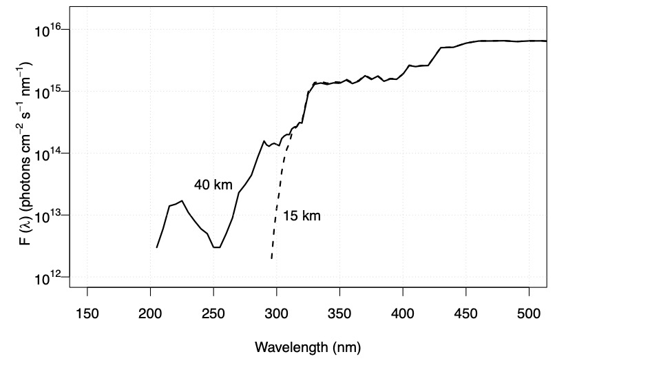
Fig. 4.60 Wavelength dependence of incident radiation at two altitudes (40 km and 15 km) on Earth.

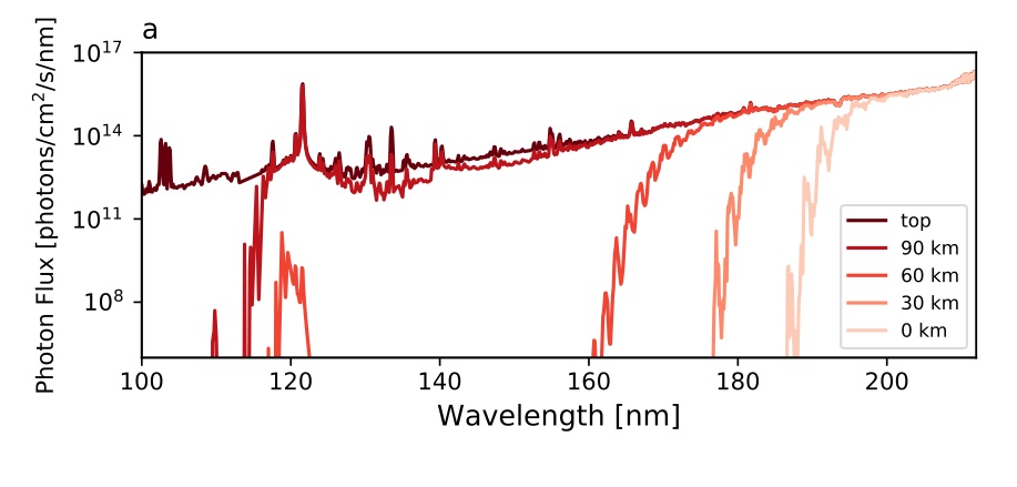
Fig. 4.61 Wavelength dependence of incident radiation at five altitudes on Mars.

These altitude dependencies of photon fluxes are important for when we come to calculate the photolysis rates of compounds in different parts of an atmosphere. Fig. 4.60 highlights that at 290 nm there is a difference of a factor of 100 in the flux of photons between 40 km and 15 km on Earth. Hence, processes requiring this wavelength of radiation will proceed much slower at 15 km than 40 km on Earth. Fig. 4.61 shows that at 200 nm there is essentially no change in the flux of photons from the top of the atmosphere to the surface of Mars.

Photolysis of O\(_2\)

The presence of O\(_2\) has a profound effect on the photochemistry of an atmosphere. O\(_2\) is likely to have been present in our atmosphere for the last 2 billion years, with the current mixing ratio of O\(_2\) roughly constant over the last 500 million years.

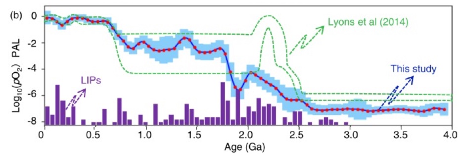
Fig. 4.62 The atmospheric history of O\(_2\) on Earth as reconstructed using geochemical proxies and machine learning (blue). After Chen et al., 2022.

O\(_2\) is produced through photosynthesis and is involved in a number of biogeochemical cycles, which give rise to long lifetimes in the lower atmosphere (thousands of years). However, in the stratosphere O\(_2\) can absorb short \(\lambda\) radiation and photo-dissociate. The absorption cross section for O\(_2\) is shown in Fig. 4.63 and consists of some characteristic features, many named after the scientists that discovered them. The absorption cross section at \(\lambda < 150\) nm is large but not important to O\(_2\) photolysis in Earth’s stratosphere owing to a lack of photons at these wavelengths. The major absorption in Earth’s stratosphere is in the Herzberg continuum (220-260 nm).

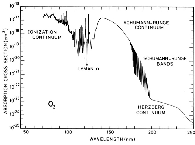
Fig. 4.63 Molecular oxygen absorption cross sections.

If we make the assumption of unit quantum yield for photolysis of O\(_2\):

\[ {\rm O_2} + h\nu \rightarrow {\rm O(^3P) + O(^3P)} \]

We can use the information in Fig. 4.60 and Fig. 4.63 to calculate the photolysis frequencies of O\(_2\) (\(J_{\rm O_2}\)). If we take the reciprocal of these frequencies we can then determine the life-times or time scales for photolysis. \(J\) values for O\(_2\) from the individual absorption bands and integrated over all \(\lambda\) are shown in Fig. 4.64.

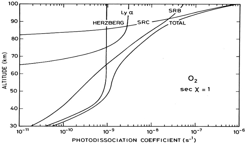
Fig. 4.64 Contribution of different bands to the photolysis of molecular oxygen

As we can see from Fig. 4.64, the lifetime of O2 with respect to photolysis varies over 5 orders of magnitude over the altitude range 100-20 km. Note that the longer wavelength Herzberg absorption is relatively more important at low altitudes while the shorter wavelengths (Schumann-Runge Bands, Schumann-Runge Continuum) are only important at high altitudes (photons at these wavelengths are absorbed high up).

Chemical reaction networks

Now we know the processes that species undergo in an atmosphere we can start to put together a network of reactions which maps out the chemistry of an atmosphere.

The development of chemical reaction networks is complex but we can break it down into a series of protocols.

1. List out all the species that are observed in an atmosphere

2. Apply reaction rules to these species to list out the possible reactions that could take place

3. Search kinetic databases or use theoretical approaches to determine the rate coefficients for each reaction

4. Compare the predictions from the network with observations and refine network parameters

Reaction rules for atmospheric chemistry

Reactions in an atmosphere occur through either collisions or absorption of photons.

When two species collide there are a limited number of outcomes. Let’s consider an example of an A molecule colliding with a BC molecule.

\[\begin{split} \begin{align} \mathrm{\mathbf{Addition:}}&\\ {\rm A + BC} &\rightarrow {\rm ABC}\\ \mathrm{\mathbf{Abstraction:}}&\\ {\rm A + BC} &\rightarrow {\rm AB + C}\\ {\rm A + BC} &\rightarrow {\rm AC + B} \end{align} \end{split}\]

As our molecules get more complex (include more atoms) then the number of possible products increases considerably.

For absorption of photons we can consider photolysis (breaking of bonds), excitation (increasing energy levels) or rearrangement. Let’s consider another example of a molecule ABC.

\[\begin{split} \begin{align} \mathrm{\mathbf{Photolysis:}}&\\ {\rm ABC} + h\nu &\rightarrow {\rm A + BC}\\ {\rm ABC} + h\nu &\rightarrow {\rm AB + C}\\ \mathrm{\mathbf{Photo-excitation:}}&\\ {\rm ABC} + h\nu &\rightarrow {\rm ABC^*}\\ {\rm ABC^*} &\rightarrow {\rm ABC} + h\nu\\ \mathrm{\mathbf{Rearrangement:}}&\\ {\rm ABC} + h\nu &\rightarrow {\rm ACB}\\ {\rm ABC} + h\nu &\rightarrow {\rm BCA}\\ {\rm ABC} + h\nu &\rightarrow {\rm BAC} \end{align} \end{split}\]

We won’t dwell on ionisation reactions in these lectures but note that they add considerable further complexity. Generally speaking these reactions are only of importance in the upper atmosphere of a planet.

Using these rules and applying them to all the known species in an atmosphere can lead to a large number of reactions to consider in our network. The next challenge is to then simplify these networks for numerical simulation.

Simplifying reaction networks

Reaction networks describe how the different constituents of the atmosphere (the gases and aerosols) react. They are also sometimes called “mechanisms” as they provide a mechanism to go from some reactant molecules to some products.

Consider a very simple reaction network involving seven species (A-G) undergoing three reactions:

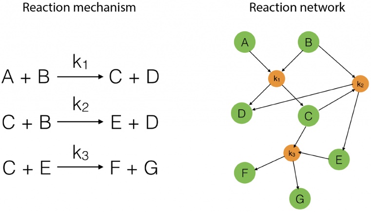
Fig. 4.65 A schematic showing how we can go from a list of reactions (a mechanism) to a reaction network viewed as a graph. Reproduced from NetworkPages.

As we can see from Fig. 4.65, we can appeal to mathematical graph theory when thinking about reaction networks, with the species being nodes on the graph and the reactions being the vectors between the nodes.

By considering the reaction network as a graph we can start to “work on it” to reduce the number of vectors and nodes needed to “map out” the reaction space. We won’t go into the details of this.

The biggest challenge with simplifying the reaction network is that the connectivity of the network is state dependent. That is as we change the conditions under which the reactions we have listed out are taking place, some will become more or less important.

Again, let’s consider an example, this time from some work from Paul and Oli.

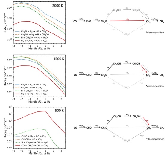
Fig. 4.66 Reaction rates as a function of fO2 and temperature highlighting that under different conditions different reactions in the network become dominant. Modified after Liggins et al., 2023.

The overall network is shown in Fig. 4.66 on the right hand side panels and in red we can see how changing the conditions the network is subjected to change the main pathways to go from the CO reactant to the CH4 product (using bold lines and red to identify the rate limiting step).

This state dependence causes a real problem for modelling the chemistry of an atmosphere and in general I would suggest that in the first instance generate as complex a network as you can and then be guided by its performance against observations before trying to simplify it.