Understand the concept of reaction rates, and kinetically and thermodynamically driven reactions.
Become familiar with Potential Energy Surfaces
Understand the concept of a transition state
Use Transition State theory to understand what dictates the rate of a reaction
The goal of this lecture is to dig into some more details of how and why a chemical reaction happens. This subject has deep theoretical foundations in statistical mechanics and can involve a lot of mathematical detail, but here I will present it with as little maths as possible. Mathematical details can be found in more advanced textbooks.
Introduction to rates
We will start by analysing a simple bimolecular reaction (made up from three atoms, A, B, and C, initially as molecules A and BC).
\[\ce{A + BC -> AB + C}\]
You have already seen that, in isolation, after a long period of time an equilibrium is reached:
\[\ce{A + BC <=> AB + C}\]
Once an equilibrium has been reached, the extent of this reaction is be determined by its equilibrium constant
NB the Gibbs free energy of each of the individual substances is temperature dependent, so \(\Delta_r G^\ominus\) will also be temperature dependent.
The various factors which determine \(\Delta_r G^\ominus\) can be calculated from statistical thermodynamics from the molecular energy levels (through the partition function), and so for simple molecules, can in principle be determined computationally. In the simple case of a gas-phase molecule, these energy levels are governed by the rotations and vibrations of the molecule and can be accurately measured by microwave and infrared spectroscopy.
In the literature, you may find a common approximation replacing the activities of a substance in solution by its concentration. This is not strictly dimensionally correct, and instead we may write
\(a_X \approx \frac{[X]}{c^0}\)
where \(c^0\) is a standard concentration (e.g. \(\pu{1 mol dm-3}\)). This approximation is good in the low concentration limit, and we will make use of it throughout this lecture.
In general, however, a system is not as a whole at equilibrium, so it is helpful to also look at the time dependence of chemical reactions, a field called chemical kinetics. If the timescale of a reaction is fast compared to our observations, and the reaction reaches equilibrium, we say it is ‘thermodynamically controlled’. If, however, the reaction is slow compared to observation, and we do not readily reach equilibrium, it is ‘kinetically controlled’.
In gases and liquids, molecules are colliding all the time, and some of these collisions lead to a chemical reaction.
In general collisions involving more than two molecules at a time are unlikely and we will consider the case of a bimolecular reaction.
Elementary reactions.
A complicated reaction can usually be broken down into a sequence of elementary reactions where (usually) two molecules collide to form products
The rate law for an elementary step relates the rate of that reaction to the concentration of the reactants
For [1] every time the reaction proceeds two molecules of \(\ce{NO}\) are needed (so \([\ce{NO}]^2\)) and 2 moles of \(\ce{NO}\) are used up and 1 mole of \(\ce{N2O2}\) is produced. \(\frac{d[\ce{NO}]}{dt} = -2 k_1 [\ce{NO}]^2\) and \(\frac{d[\ce{N2O2}]}{dt}= k_1[\ce{NO}]^2\).
For [2], e.g. \(\frac{d[\ce{O2}]}{dt}= -k_2[\ce{N2O2}][\ce{O2}]\).
The overall rate of reaction (e.g. \(\frac{d[\ce{NO2}]}{dt}\)) can be determined by coupling the individual rate equations together, and this will be explored in later lectures.
Here we shall look at the factors which control the rates of the individual elementary reactions.
Reaction Pathways
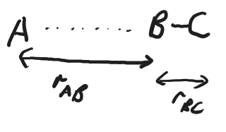
To understand what occurs during a chemical reaction we can look at the energy of the combined system of reactants as a function of the positions of the atoms. Even in our three-atom, two molecule system, that is far too many degrees of freedom to plot, so we will consider the simple case of one dimension, where A, B, and C are collinear, with distances, \(r_\ce{AB}\) and \(r_\ce{BC}\).
Fig. 4.36 Diagram of bimolecular reaction of A and BC in collinear orientation.#
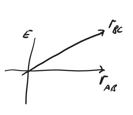
It is possible to plot the ‘energy’ of the system as a function of these two coordinates. This diagram is usually called a Potential Energy Surface (PES), as it describes the potential energy of the system as a function of the atomic positions. (This ‘Potential energy’ of course includes the effects of chemical bonding, including the kinetic energy of the electrons. More formally in thermodynamics, it is the ‘internal energy’, \(U\).)
Fig. 4.37 A 3-dimensional plot of a Potential energy surface with coordinates \(r_\ce{AB}\) and \(r_\ce{BC}\) is too difficult to draw.#
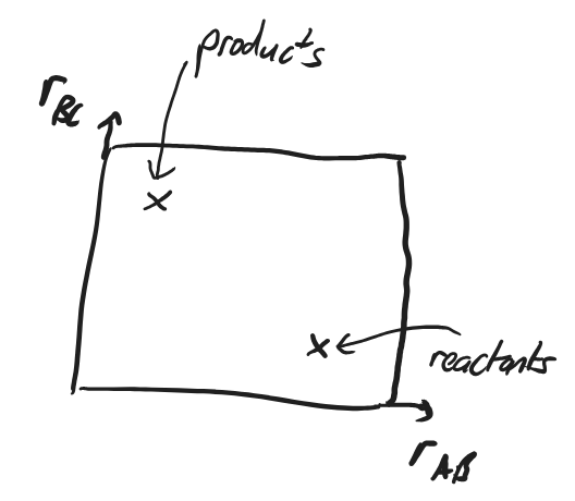
The reactants, if they are stable, will sit in a local minimum of the PES with a large \(r_\ce{AB}\) and short \(r_\ce{BC}\). (Because the molecules are themselves quantum mechanical, they don’t just sit at the minimum of this well. Their (nuclear) wavefunction is spread over the minimum of the PES.).
Similarly the products will sit in a different local minimum with a (probably) different energy.
Fig. 4.38 A 2-dimensional plot of the reaction space with coordinates \(r_\ce{AB}\) and \(r_\ce{BC}\), showing the position of reactants and products.#
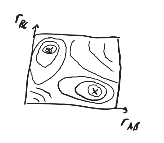
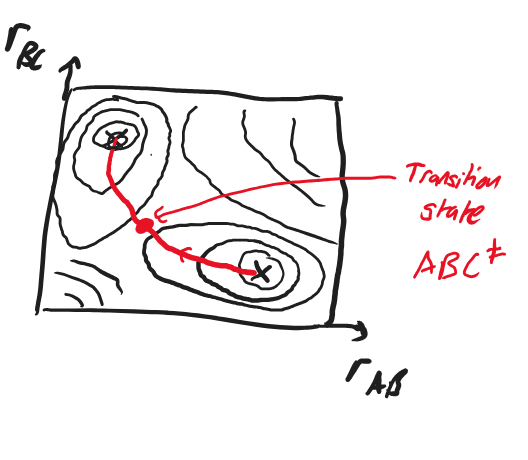
Fig. 4.39 A 2-dimensional contour plot of the energy in the reaction space with coordinates \(r_\ce{AB}\) and \(r_\ce{BC}\), showing the reactants and products as local minima.#
We describe a chemical reaction by a pathway on the PES joining the reactants minimum with the products minimum.
Fig. 4.40 A 2-dimensional contour plot of the energy in the reaction space with coordinates \(r_\ce{AB}\) and \(r_\ce{BC}\), showing the reactants and products as local minima joined by their reaction pathway containing the transition state \(\ce{ABC^\ddagger}.\)#
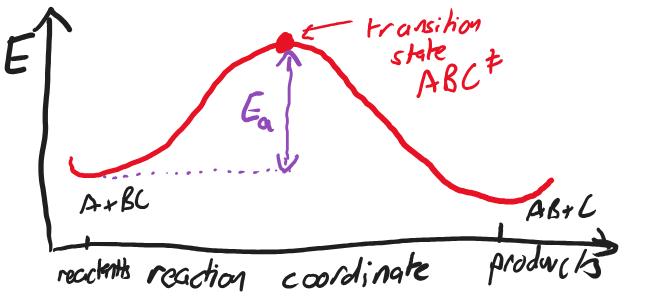
We can more conveniently plot the energy along the pathway from reactants to products as in the figure below.
Fig. 4.41 A plot of the energy in the against reaction coordinate, showing the highest energy point, the transition state, and the activation energy.#
The maximum on this pathway is known as the transition state, and it is this configuration which usually dictates the speed of the reaction.
The simplest model using this concept is the Arrhenius Equation, where it is assumed that to overcome the barrier for the reaction to proceed, an Activation Energy, \(E_a\) is required. At a temperature, \(T\), the relative likelihood of gaining activation energy \(E_a\) is given by the Boltzmann Factor, \(\exp(-E_a/RT)\), and so the Arrhenius Equation is born:
\[k = A e^{\frac{-E_a}{RT}}.\]
Many reactions approximately fit this, though the equation it is not directly based in statistical thermodynamics.
Instead we can use an approach called “Eyring Transition State Theory”. We assume that the reaction proceeds through the transition state labelled \(\ce{ABC}^\ddagger\).
Since the transition state is significantly higher in energy than the reactants, relatively few collisions of \(\ce{A + BC}\) reach the transition state, and so we can statistically model the few that do. This is done by assuming that the reactants and transition state are in equilibrium, with equilibrium constant \(K^*\).
\[\ce{A + BC <=> ABC^\ddagger -> AB + C}\]
Further, we assume that once a system has reached the transition state, it has a fixed rate of descending the PES to the reactants, \(k_\text{1st}\).
Since the reaction is overall second order, \(\text{rate} = k_\text{2nd} [\ce{A}][\ce{B}]\),
so we may read off that \(k_\text{2nd} = k_\text{1st} \frac{K^*}{c^0}\).
Since the equilibrium to the transition state is thermodynamically controlled, \(K^*\) is determined by the free energy difference between reactants and the transition state. Because, however, the transition state is not a local minimum, and approximation must be used which factors out the motion along the reaction co-ordinate (where is it a local maximum). We can designate a ‘vibrational’ frequency along this co-ordinate as \(\nu^\ddagger\), leading to
The remaining factors which determine \(\Delta G^\ddagger\) be calculated from computationally with calculations of both the reactants’ local minimum and the transition state structure (explicitly ignoring the vibrational mode which crosses over the transition state in the latter).
All that remains is to now determine \(k_\text{1st}\). A slight sleight of hand allows us to equate it to \(\nu^\ddagger\) (which is the ‘frequency’ of vibrations crossing the transition state), resulting in overall rate equation
There are two sources of temperature dependence, giving rise to what looks like a disagreement with the Arrhenius Equation.
However, if we interpret the activation energy as a temperature dependent quantity, we may attempt to match these equations (this is done via considering the partial derivative \(\frac{\partial \ln{k_\text{2nd}}}{ \partial\frac{1}{T}}\)), giving
\(E_a = \Delta H^\ddagger + 2RT\) for bimolecular gas phase reactions and
\(E_a = \Delta H^\ddagger + RT\) for solution and unimolecular gas phase reactions.
\(RT\) is generally a relatively negligible, and \(E_a\) is dominated by \(\Delta H^\ddagger\).
We also see that the pre-exponential factor is both temperature dependent, and has a significant entropic component. In the gas phase, when two molecules collide, there is a significant reduction in entropy in the transition state. In solution-phase reactions, the free energy (and thus the enthalpy and entropy) for the transition state includes all the often very significant solvent effects, and these may act to enhance or decrease entropies of reaction. In general if the magnitude of charges are increased (e.g. \(\ce{AB -> ^{\delta+}A...B^{\delta-}}\)) this leads to significantly negative entropies of activation.
Not all chemical reactions occur from molecules in their ground state, owing to often large activation energy barriers. One way of overcoming this is to first excite a molecule to a higher energy electronic state, usually by the absorption of a photon. This may then react or decompose.
This process involves two PESes: the ground state of \(\ce{X}\) which may have a high barrier to producing \(\ce{A+B}\), and its excited state, \(\ce{X^*}\), where it’s possible that making the products is even exothermic.
You can envisage the PESs for such a process.
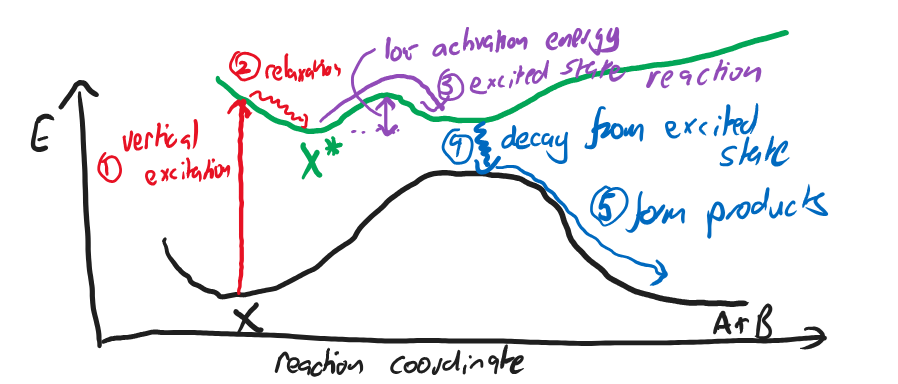
Fig. 4.42 A plot of the potential energy surfaces of ground and excited states, and a possible excited state pathway to the products.#
In this figure a typical excited state reaction is given:
Molecule X in its ground state absorbs a photon and excited to its excited state PES. Typically the molecule is no longer at a minimum of this new PES.
The molecule relaxes to a local minimum of the PES.
The molecule overcomes the small barrier towards the products in the excited state
The molecule releases energy (e.g. by giving out a photon or by a collision) to move it to its ground state PES.
The molecule moves down the ground state PES to the products.
In general PESs do not often cross, and instead smoothly switch character as the nuclear coordinates change. For reactions where there are significant changes in electronic structure this can lead to signficant barriers. Occasionally, the PESs of different electronic states will cross at a point of accidental degeneracy. Such points are known as conical intersections and are very significant in the relaxation processes of excited state reactions.
Note that in general the different spin states of atoms and molecules lie on different PESs (which can cross), and so a reaction which does not preserve spin is known as spin-forbidden. Changing the spin state requires siginificant spin-orbit coupling, and this generally does not occur in molecules with first-row atoms, but is increasingly likely with heavier atoms.