2.11. Debris disks I: Physical Structure#
Professor: Mark Wyatt (IoA)
Learning objectives:
What a debris disk is.
The components of the Solar system’s debris disk, such as the Kuiper belt.
How debris disks are detected around other stars.
Collisional cascades: how asteroids get ground down to dust.
The structure of debris disks from images.
The diverse population of debris disks, including exo-Kuiper belts and exozodi.
The aim of this lecture is to understand the components of planetary systems that are not planets, collectively known as a star’s debris disk. This lecture will describe what we know about the Solar system’s debris disk and how we get information about the debris disks of other stars. It will describe the underlying physics needed to understand processes going on in the disks, and what we know about the structure and evolution of extrasolar debris disks.
What is a debris disk?#
There are two perspectives on what a debris disk is:
(i) Probably the most helpful is to consider a debris disk as being made up of the components of the star’s planetary system that are not planets. Thus debris disks are comprised of the system’s asteroids and comets (collectively called planetesimals, or minor planets), as well as the dust and gas that arises in the destruction of those bodies.
(ii) The other perspective is to consider them as the descendent of the star’s protoplanetary disk. This definition arises because a protoplanetary disk also satisfies the condition in (i), in that it is made up of circumstellar material that isn’t a planet. There is no good way to distinguish between a protoplanetary disk and a debris disk, although a rule of thumb is that the former have lots of gas and dust and are found around young stars <<10Myr, whereas the latter are found around older stars >>10Myr and have modest levels of dust and usually little gas.
The Solar system’s debris disk#
The Solar system’s debris disk is made up of (see Fig. 2.70):
the asteroids in the Asteroid Belt orbiting at 2-3.5au from the Sun, the largest of which is Ceres at ~950km diameter;
the Trans-Neptunian Objects in the Kuiper Belt orbiting at 30-40au from the Sun, the largest of which is Eris at ~2400km diameter;
the comets in the Oort Cloud, at 10,000-100,000au from the Sun.
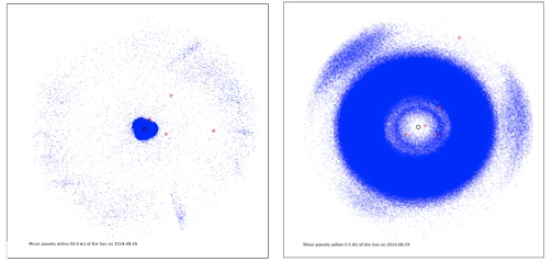
Fig. 2.70 Spatial distribution of the known minor planets in the Solar system (see www.minorplanetcenter.net ): left – view out to 50au, right – zoom in to 5.5au. The locations of planets are shown with red circles.#
These populations reside in all locations in the Solar system where an object could survive 4.5Gyr of evolution given that their orbits are subject to gravitational perturbations from the planets. Indeed, the dynamical structure of these populations (i.e., the distribution of orbits of the bodies) shows this in exquisite detail. For example, the asteroid belt is bounded by secular resonances, and has narrow Kirkwood gaps associated with Jupiter’s mean motion resonances.
There are many further classes of object which are short-lived and so derive from the long-lived populations, such as:
the Near Earth Objects, which are asteroids that have been nudged out of the Asteroid Belt (likely by a radiation force known as the Yarkovsky force combined with gravitational interactions with planets) so that they now orbit <2au, some of which may end up on a collision course with the Earth;
the Jupiter Family Comets, which are TNOs which have been nudged out of the Kuiper belt to orbit <30au, most of which are ejected from the Solar system by Jupiter, but some of which reach the inner Solar system where they are heated releasing gas and dust;
the Zodiacal Cloud, which is the dust disk within which the Earth sits, extending from the Sun out to at least 4au, although dust extends all the way out to the Kuiper belt, which is replenished by the break-up of asteroids and comets.
All populations are made up of many objects that form a size distribution. This distribution is usually close to a power law so that if \(n(D)dD\) is the number of objects in the size range \(D\) to \(D+dD\) then \( n(D) \propto D^{-\alpha}\), where \(\alpha\) is close to 3.5. In such a distribution most of the mass is in the largest objects, while most of the cross-sectional area is in the smallest objects. While the largest objects are known, in general the smallest (below 100s of m to 10s of km, depending on distance) are too faint to detect individually. This is not true for the zodiacal cloud for which it is usually the collectively large cross-sectional area of the smallest dust which renders it detectable. For example, sunlight scattered by the dust can be seen with the naked eye as the zodiacal light, while thermal emission from this dust (due to it being heated when absorbing radiation from the Sun), makes the zodiacal cloud the brightest object in the infrared sky.
How are extrasolar debris disks discovered?#
The vast majority of extrasolar debris disks are discovered not by detecting individual large minor planets, rather by detecting the collective effect of many dust grains that have been created in the destruction of those bodies (see Wyatt 2008). That is, they are detected by their component that is analogous to the zodiacal cloud. They are usually discovered due to the thermal emission from the dust which is heated by the star and reradiates that emission in the infrared.
Let us assume the dust resides in a belt at a radius \(r\) from a star of luminosity \(L_\star\) and has a total cross-sectional area \(\sigma_{\rm tot}\). If the dust interacts with stellar radiation like a black body (i.e., absorbing all the incident radiation) then energy balance shows it will be heated to a temperature:
\( T = 278 L_\star^{1/4} r^{-1/2}, \)
where \(r\) is in au, \(L_\star\) in \(L_\odot\) and \(T\) in K. The disk’s brightness is often expressed in terms of the fractional luminosity of the dust, \(f=L_{\rm dust}/L_\star\), i.e., the ratio of the disk luminosity to that of the star. Since all the energy absorbed by the dust is re-emitted, geometrical arguments show that the fractional luminosity of the dust emission is given by
\( f = \sigma_{\rm tot} / (4 \pi r^2). \)
Fig. 2.71 shows the spectrum of a star with a debris disk. This illustrates how a debris disk can be much brighter than the star at wavelengths \(>10\mu\)m, as long as the fractional luminosity is not too low. Thus debris disks are discovered by looking at a star and performing photometry (i.e., determining the total flux density at a given wavelength), and determining whether the star exhibits excess emission. Excess in this context means an excess above that expected from the stellar photosphere alone, which can usually be predicted to within a few % from observations at shorter wavelengths where no dust emission is expected. Thus to be discovered a debris disk has to both be bright enough to detect (given the sensitivity of the instrument observing it) and to be bright relative to the star to ascertain that we are not just seeing the star.
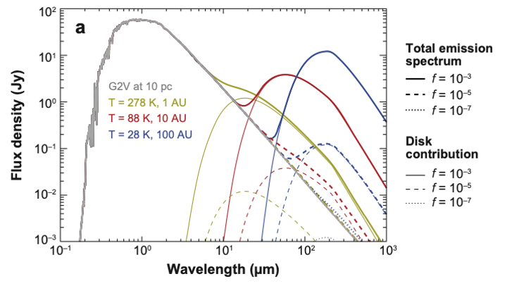
Fig. 2.71 Spectral energy distribution (SED) of a Sun-like star with a debris disk comprised of dust all at the same distance from the star (from Wyatt 2008). The dust is assumed to act like a black body. Emission from the star itself (i.e., its photosphere) is shown with the grey line, while the coloured lines of different styles show the contribution of debris disks at different distances from the star (1, 10, 100 au) and of different fractional luminosities (\(10^{-3}\), \(10^{-5}\), \(10^{-7}\)).#
Debris disk physics#
Most objects in a debris disk simply orbit the star until they collide with another object. Most collisions are with much smaller objects that are inconsequential. Collisions with large objects (meaning similar in size or larger), on the other hand, are important since they result in the object being destroyed and its mass turned into smaller objects. Such collisions are called catastrophic, and since collisions with much larger objects are rare, it is collisions with similar-sized bodies that are most important. In this way a collisional cascade is set up, wherein large objects collide creating smaller fragments, which themselves collide creating even smaller fragments, until the mass is ground down into dust at which point radiation forces become important. It can be shown that for minimal assumptions this collisional cascade leads to a size distribution with \(\alpha=3.5\) as observed (Wyatt et al 2011).
Radiation forces are quantified by the \(\beta\) parameter, which is the ratio of this force to the gravitational attraction of the star. For black body dust of diameter \(D\) in \(\mu\)m, this is
\( \beta \approx 0.4 (L_\star/M_\star) / D, \)
where stellar luminosity and mass are in solar units and a density of 2700kg/m\(^3\) has been assumed for the dust. There are two components to radiation forces:
There is a drag force opposing the motion called Poynting-Robertson drag, which causes the dust to migrate in towards the star. Starting from a circular orbit at a distance \(a\) in au, a dust grain would reach the star (where it would sublimate) on a timescale
\( t_{\rm pr} = 400 a^2 / (M_\star \beta), \)
in years.
The other component is purely radial, and is called radiation pressure. It is straight-forward to see that dust with \(\beta>1\) must be unbound from the star, since the outward radiation pressure is stronger than stellar gravity. However, dust released from a parent body on a circular orbit is unbound if \(\beta>0.5\), and that with \(\beta\) in the range 0.1-0.5 is put on orbits that extend far beyond the belt.
Fig. 2.72 summarises the expected size and spatial distribution of dust created in a planetesimal belt due to collisions and radiation forces (see Wyatt 2009). The largest debris forms the collisional cascade, but this cascade is truncated when the dust becomes small enough to either be dragged in toward the star or expelled by radiation pressure. Which of these mass loss mechanisms dominates is determined by the density of the belt: for high density belts like those found around other stars P-R drag does not have time to move the dust very far before it is destroyed in a collision and blown away by radiation pressure. However, in the tenuous debris disk of the Solar system, even 100\(\mu\)m dust usually gets dragged into the Sun without suffering a collision.
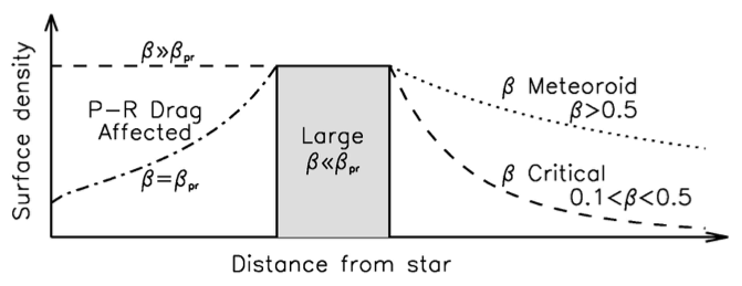
Fig. 2.72 Schematic of the surface density of dust of different sizes in a debris disk in which dust is created in a planetesimal belt (the shaded region). The largest bodies remain confined to the planetesimal belt. The smallest dust (\(\beta\) meteoroids) is blown out by radiation pressure as soon as it is created, while small bound dust (\(\beta\) critical dust) is placed in a halo outside the belt. If the disk is tenuous enough a component of dust is dragged in towards the star where it sublimates, however it may be depleted in collisions on the way in.#
More detailed characterization of debris disks#
Basic information about a debris disk can be gleaned even from limited photometry. For example, consideration of Fig. 2.71 shows that measurements at 2 wavelengths can be used to determine the temperature and fractional luminosity of the emission. From the temperature an estimate of the radial location can be made. However, we would have had to assume the spectrum is that of a black body and that the dust acts like a black body. From the fractional luminosity the cross-sectional area in dust can be estimated, from which the total mass can be estimated, but such a calculation would have to assume a size distribution and maximum planetesimal size.
Fortunately there are many observational techniques to get additional information about debris disks:
Imaging#
Since debris disks are found around the stars nearest to the Sun, this means that the spatial extent of their debris disks are often large enough to be directly imaged.
At the longest wavelengths (\(>30\mu\)m) the disk’s thermal emission is brighter than the star, and so imaging of a disk at these wavelengths simply requires sufficient sensitivity. Since debris disks are faint, this is still challenging. However, around 100 debris disks have been imaged at sub-mm wavelengths (e.g., Hughes et al. 2018).
At shorter wavelengths (\(<5\mu\)m) where scattered light dominates, sensitivity is still a challenge, but there is the additional problem of having to subtract the emission of the bright star (e.g., Ren et al. 2023). This is similar to the problem of directly imaging exoplanets, except the challenge is greater to disentangle a diffuse disk structure from stellar emission. Stellar subtraction can be achieved by coronagraphic techniques (to block the starlight) or by using interferometric techniques.
The first disk to be imaged was that of the star \(\beta\) Pictoris, which was helped by this being particularly young (and so high fractional luminosity) and nearby (and so both bright and large on the sky), and also edge-on (resulting in a high surface brightness and facilitating disentangling from stellar emission). This has now been imaged at multiple wavelengths as shown in Fig. 2.73.
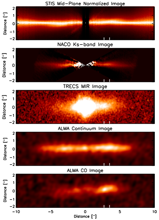
Fig. 2.73 Images of the \(\beta\) Pictoris debris disk at multiple wavelengths (Apai et al. 2015). The optical (STIS) and near-IR (NACO) images trace scattered light from the debris disk and have had the star itself blocked by coronagraphy. The stellar emission has not been removed from the mid-IR (TRECS) and sub-mm (ALMA) images which trace the disk’s thermal emission. The lower image traces CO gas in the disk.#
Disk imaging can be (and has been) used to reveal:
The radial location of the planetesimal belt and its width (e.g., indicating the range of distances over which planetesimals were able to form in the protoplanetary disk and/or how their distribution was shaped by planets)
The sharpness of a disk’s edges (which if sculpted by a planet reveals its properties)
Gaps in the disk (possibly indicating the location of unseen planets)
Vertical structure (indicative of the dynamical processes stirring the disk)
Warps (due to secular perturbations from the planetary system; see STIS image in Fig. 2.73
Clumps (due to recent collisions or resonances with planets; See TRECS image in Fig. 2.73)
Eccentricities (due to perturbations from eccentric planets or binary companions).
Spectroscopy#
Spectroscopy is simply a method of taking multiple photometric measurements. This means that even with low (wavelength) resolution it is possible to test how closely the emission resembles a black body. At higher resolution more subtle features of the spectrum can be gleaned, while at the highest resolution it is possible to detect the lines of emission from specific gases. We will return to this in the next lecture.
The diverse debris disk population#
Exo-Kuiper Belts#
By now several 100s of candidate debris disks are known in varying states of characterization. The majority were discovered during far-IR surveys at wavelengths of \(24-160\mu\)m, revealing a population of extrasolar analogues to the Kuiper belt that are detected to ~20% of stars (see Wyatt 2020). Fig. 2.74 summarises the results of such surveys of nearby stars. The disks all lie in a well defined part of the fractional luminosity – radius plot that can be readily understood:
There is a lower limit to the location where debris disks can be found, since those with too low fractional luminosity would be too faint to distinguish easily from their star (see Fig. 2.71). This would be the case, for example, if we had been trying to detect the Solar system’s Kuiper belt around another star.
The upper limit for large disks (\(>30\)au) arises because of a constraint on the realistic levels of mass that may be present in planetesimals, which is limited to of order \(100M_\oplus\).
For smaller disks (\(<30au\)), the upper limit arises because stars in a volume-limited sample are old, typically a few Gyr, and this means they have been collisionally eroded, with smaller disks being collisionally eroded faster. This interpretation is supported by comparing samples of debris disks found around stars of different ages: the disks around older stars are fainter, and lower fractions are detected, as expected.
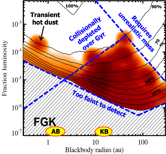
Fig. 2.74 Summary of far-IR surveys of 300 nearest Sun-like stars (i.e., those of F, G or K spectral type). The axes are the fractional luminosity and black body radius of the debris disk, and the colour scale shows the fraction of the stars that have a debris disk in different parts of this parameter space. In total 20% of stars have a detected debris disk. The disks lie between the blue dashed lines for reasons described in the text.#
Given their large size, it is this population of extrasolar Kuiper belts which has been extensively imaged. However, surveys at mid- and near-IR wavelengths have shown that there is also a population of dust much closer to the star. For some stars these two populations can be seen because their SED does not resemble a single temperature black body, rather requiring two temperature components (i.e., a hot component analogous to the zodiacal cloud and a cold component analogous to the Kuiper belt). However, in other cases the warmer component represents a small perturbation to the overall spectrum, but can spatially distinguished from the outer component by other techniques.
Exozodiacal dust#
By analogy with the zodiacal cloud, dust that is found within ~5au from the star is referred to as the star’s exozodiacal dust (or exozodi for short). Due to its temperature such dust is usually detected in mid-IR observations. As implied by Fig. 2.74, any high fractional luminosity disks found in close proximity to old stars (there are a few) cannot be explained by steady state collisional erosion of an in situ asteroid belt, since collisions would have depleted the belts over Gyr of evolution. Any such dust is inferred to be a transient phenomenon, for example created in a recent collision and thus will soon disperse. If found around a young star (\(<100\)Myr), however, such bright hot dust could be indicative of a massive asteroid belt.
There has been significant interest in exozodi from NASA for a very pragmatic reason: any dust that resides in a star’s habitable zone acts as a noise source which can prevent detection of an exo-Earth (Roberge et al. 2012; Currie et al. 2023). Or rather, since we are now in the design phase of such a mission, detection of an exo-Earth would require us to build a larger telescope to achieve the detection which translates into the billions of dollars needed to achieve this. Unfortunately the rule of thumb is that an exozodi 10 times brighter than our own zodiacal cloud (i.e., 10 zodi) would be problematic, and yet we can only detect exozodi photometrically at 1000 zodi levels. This led to the development of nulling interferometric techniques which have shown that 100 zodi levels are present at 20% of stars (Ertel et al. 2020).
These exozodi detections correlate with the presence of an outer Kuiper belt, supporting that material is being transported inwards somehow. In some systems there is evidence that points to an exocometary origin for the exozodi (e.g., planets are scattering in km-sized planetesimals), while in others the surface brightness distribution is consistent with only dust being brought in by P-R drag. The exozodi population is discussed further in the next lecture 2.12.
Hot dust#
A surprising result from near-IR interferometry is that 20-30% of stars seem to exhibit near-IR emission from dust close to the star at ~1000K (Absil et al. 2021). This result is surprising because the detections are independent of other properties (like stellar type) and require significant quantities of dust resulting in a short collisional lifetime. Thus the dust must be continually replenished, but there is no good model to explain this, particularly since the hot dust doesn’t correlate with the presence of an outer Kuiper belt or exozodi which might be feeding that dust. Rather the lack of detection at longer wavelengths implies the dust must be very small \(\sim 100\)nm.
References#
Absil O. et al. 2021, A&A, 651, A45
Apai D. et al. 2015, ApJ, 800, 136
Currie M. H. et al. 2023, AJ, 166, 197
Ertel S. et al. 2020, AJ, 159, 177
Hughes A. M. et al. 2018, ARA&A, 56, 541
Ren, B. B. et al. 2023, A&A, 672, A114
Roberge A. et al. 2012, PASP, 124, 918
Wyatt M. C. 2008, ARA&A, 46, 339
Wyatt M. C. 2009, Lecture Notes in Physics 758, 37
Wyatt M. C. et al. 2011, CeMDA, 111, 1
Wyatt M. C. 2020, in The Trans-Neptunian Solar System, 351