3.3. Mechanisms for climate homeostasis II. Earth’s thermostat through time and the emerging view

Professor: Ed Tipper (Earth Sciences)

---

Learning Objectives:

• Marine carbonates as a proxy for seawater chemistry and climate

• Stable carbon isotopes as a tracer of the carbon cycle?

• Strontium isotopes in marine carbonates as a tracer of weathering through geological time

• Radiogenic Osmium isotopes as a tracer of petrogenic organic carbon oxidation

• The emerging view: Can weathering actually release carbon to the ocean-atmosphere system?

Maintaining an equable climate over most of the Earth’s history implies a negative feedback which regulates atmospheric \(\sf CO_2\), a key greenhouse gas. Something prevented Earth from becoming a runaway greenhouse like Venus, despite the continuous magmatic degassing over time. Silicate weathering and carbonate formation (temperature and precipitation dependent) and coupled burial of organic carbon have been cited as the major negative climate feedbacks.

Weathering reconstructed using marine carbonates as a proxy for seawater chemistry

One of the major motivations for trying to reconstruct weathering over time, is that geochemical proxies for temperature such as foraminiferal calcite show significant coherent trends. \(\delta^{18}O\) suggests that there has been significant cooling since the early Eocene. It has been proposed that this cooling is caused by increase in chemical weathering and removal of \(\sf CO_2\) from the atmopshere.

Remember: \(\sf \delta^{18}O=1000\cdot\left(\frac{\left(\frac{^{18}O}{^{16}O}\right)_{sample}}{\left(\frac{^{18}O}{^{16}O}\right)_{std}}-1\right)\)

The fractionation of \(\delta^{18}O\) in calcite is dependent on temperature:

(3.11)\[\sf T=16.9-4.38(\delta_c-\delta_w)+0.1(\delta_c-\delta_w)^2\]

Since all waters from continents end up in the oceans, the hope is that the seawater will provide a record of how continental waters have changed over time, and hence how carbon consumption from weathering has changed over time. A key area of research in the field of geochemistry is therefore to find tracers of weathering through time.

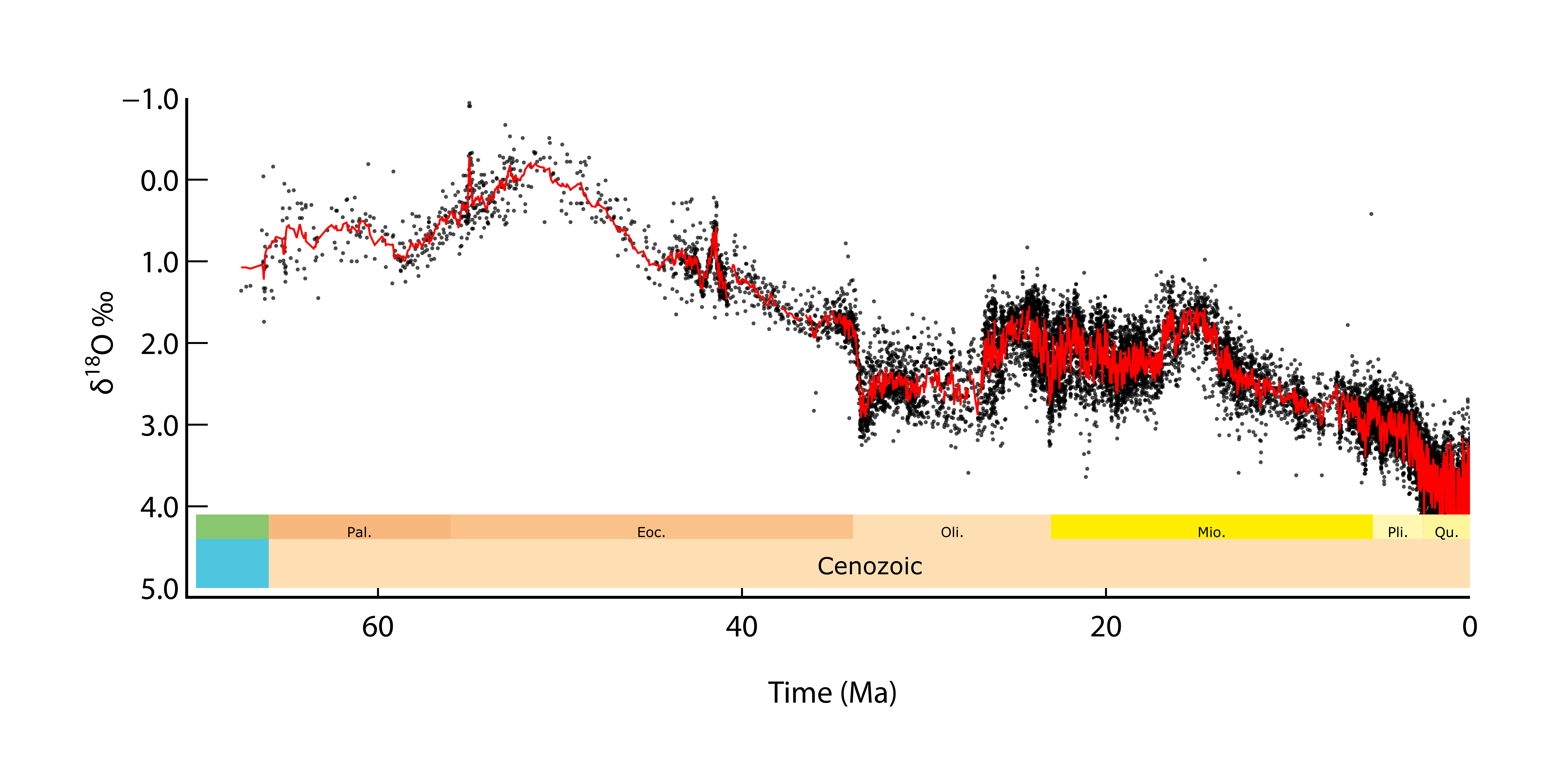
Fig. 3.26 The Cenozoic record of \(\sf \delta^{18}O\) in foraminiferal calcite, replotted from Zachos 2001. Note the reverse scale, such that \(\delta^{18}O\) varies in the same direction as T when plotted like this.

Stable carbon isotopes as a tracer of the carbon cycle?

Similar to oxygen, the element carbon has stable isotopes, and their ratio is expressed as \(\sf \delta^{13}C\).

\(\sf \delta^{13}C=1000\cdot\left(\frac{\left(\frac{^{13}C}{^{12}C}\right)_{sample}}{\left(\frac{^{13}C}{^{12}C}\right)_{standard}}-1\right)\)

Intuitively, one might expect \(\sf \delta^{13}C\) to provide a clear constraint on the carbon cycle (and greenhouse gases) over time. The reality is that \(\sf \delta^{13}C\) is complex to interpret. As a result, Earth scientists have turned to other tracers.

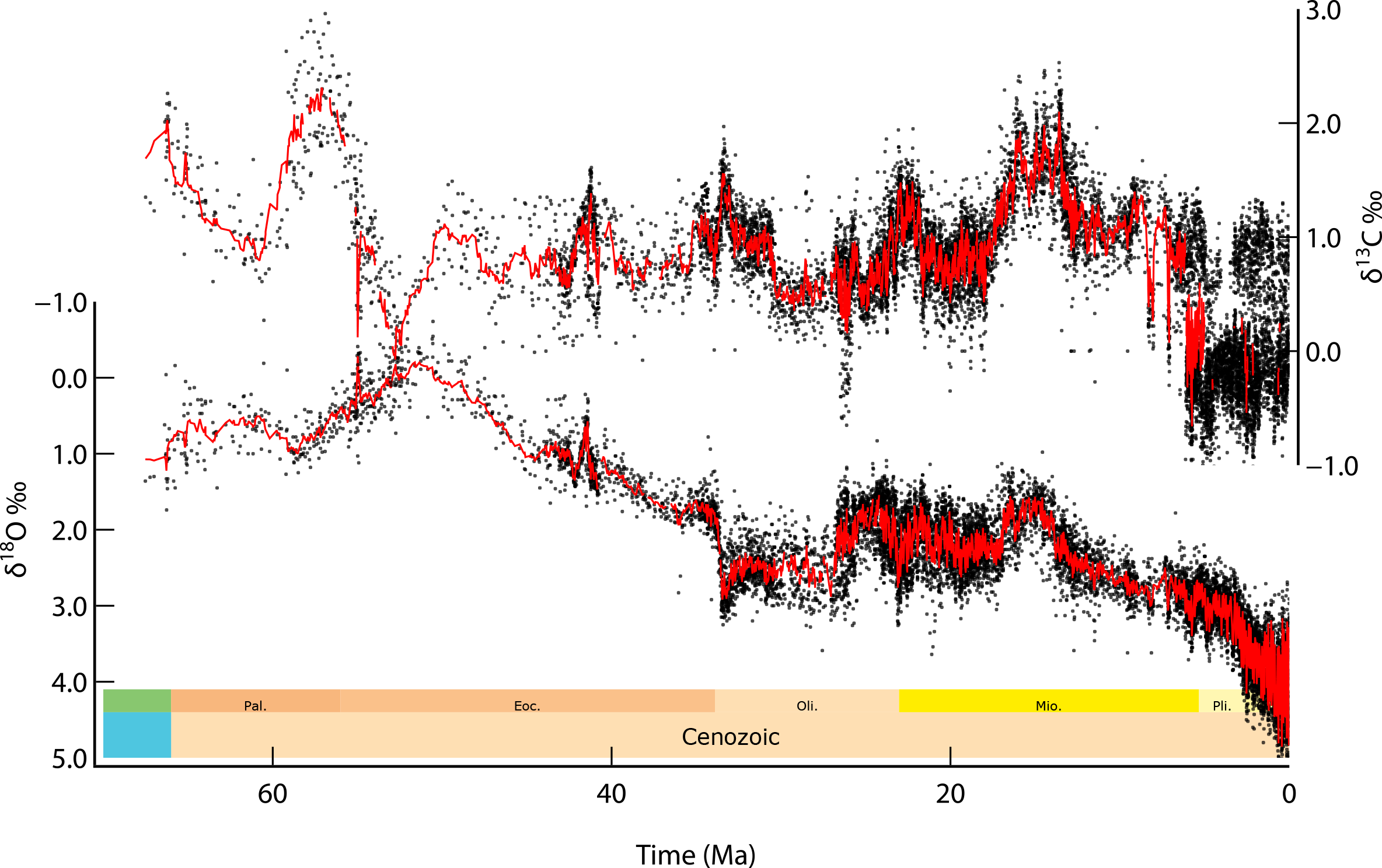
Fig. 3.27 The Cenozoic record of \(\sf \delta^{13}C\) compared with \(\delta^{18}O\) in foraminiferal calcite, replotted from Zachos 2001.

Strontium isotopes in marine carbonates as a tracer of weathering through geological time

Strontium (Sr) is a radiogenic isotope system. \(\sf ^{87}Sr\) is produced from the decay of \(\sf ^{87}Rb\) with a half life of 48.8Gyr. Sr isotope ratios are nearly always quoted as \(\sf \frac{^{87}Sr}{^{86}Sr}\). Crustal rocks are enriched in Rb because of magmatic processes. Since \(\sf ^{87}Rb\Rightarrow^{87}Sr\), the continents have a high \(\sf \frac{^{87}Sr}{^{86}Sr}\) ratio. In contrast, mantle rocks have a low Rb content, and hence have a low \(\sf \frac{^{87}Sr}{^{86}Sr}\) ratio. The reason for caring about the \(\sf \frac{^{87}Sr}{^{86}Sr}\) ratio of the mantle as part of this course is that there is a significant hydrothermal exchange between the mantle and seawater both at mid-ocean ridges and off axis hydrothermal circulation. This is summarised in the cartoon below Fig. 3.28.

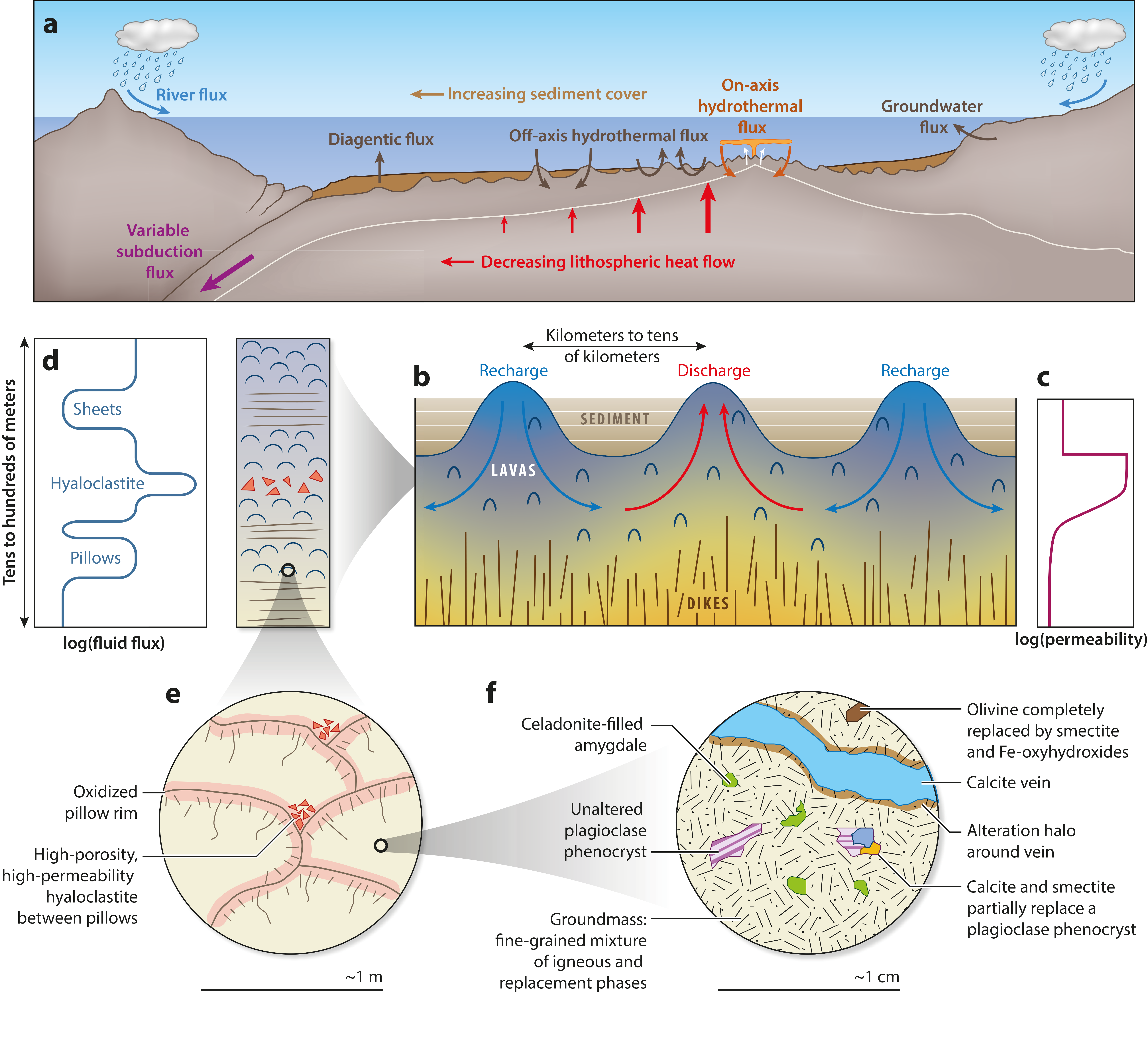
Fig. 3.28 Summary of what happens during hydrothermal circulation from Coogan et al.

In summary, hydrothermal circulation dissolves the basaltic rock, releasing Sr with a \(\sf \frac{^{87}Sr}{^{86}Sr}\) ratio of 0.703. This is in contrast to the Sr that is released during the dissolution of continental silicates with a \(\sf \frac{^{87}Sr}{^{86}Sr}\) ratio of 0.714. These two fluxes of Sr supply seawater, and mix together to give a modern seawater \(\sf \frac{^{87}Sr}{^{86}Sr}\) ratio of 0.70917. This is the modern Sr isotope budget of seawater, and it can be used to trace the relative amounts of inputs of inputs from the continents (via weathering) compared to hydrothermal circulation.

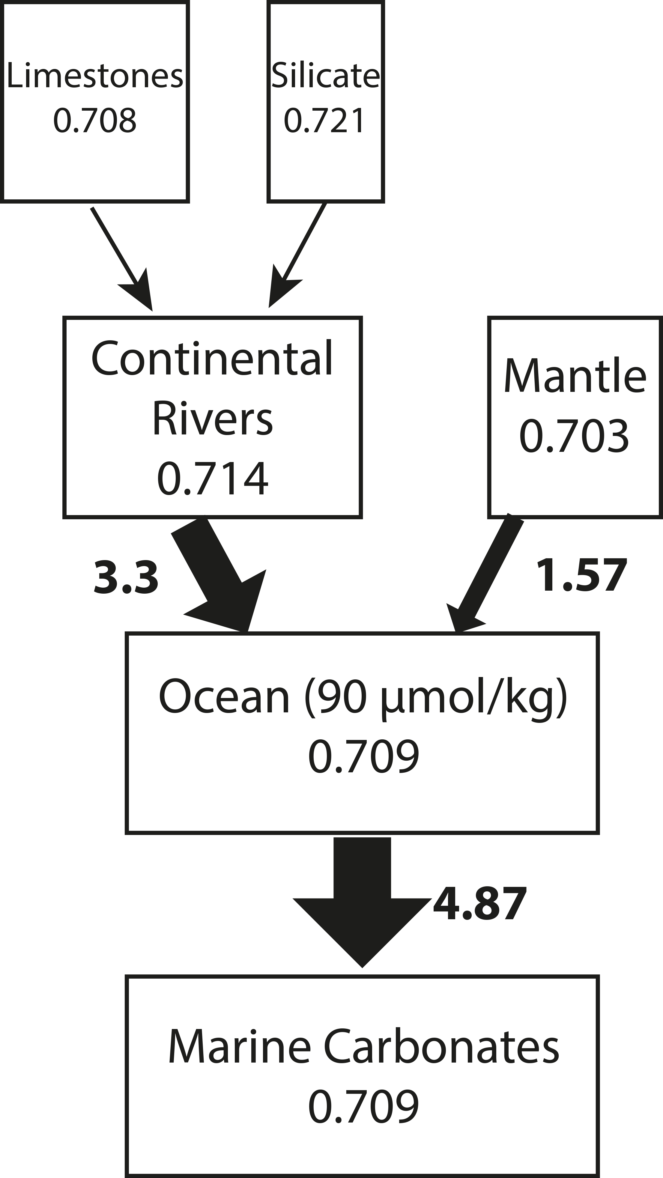
Fig. 3.29 The Sr isotope budget of modern seawater, expressed as a simple box model.

Sr (and all other chemical elements) have a residence time in the oceans. The residence time is defined by the equation:

(3.12)\[\sf \tau=\frac{N_{sw}}{J_{in}}=\frac{N_{sw}}{J_{out}}\]

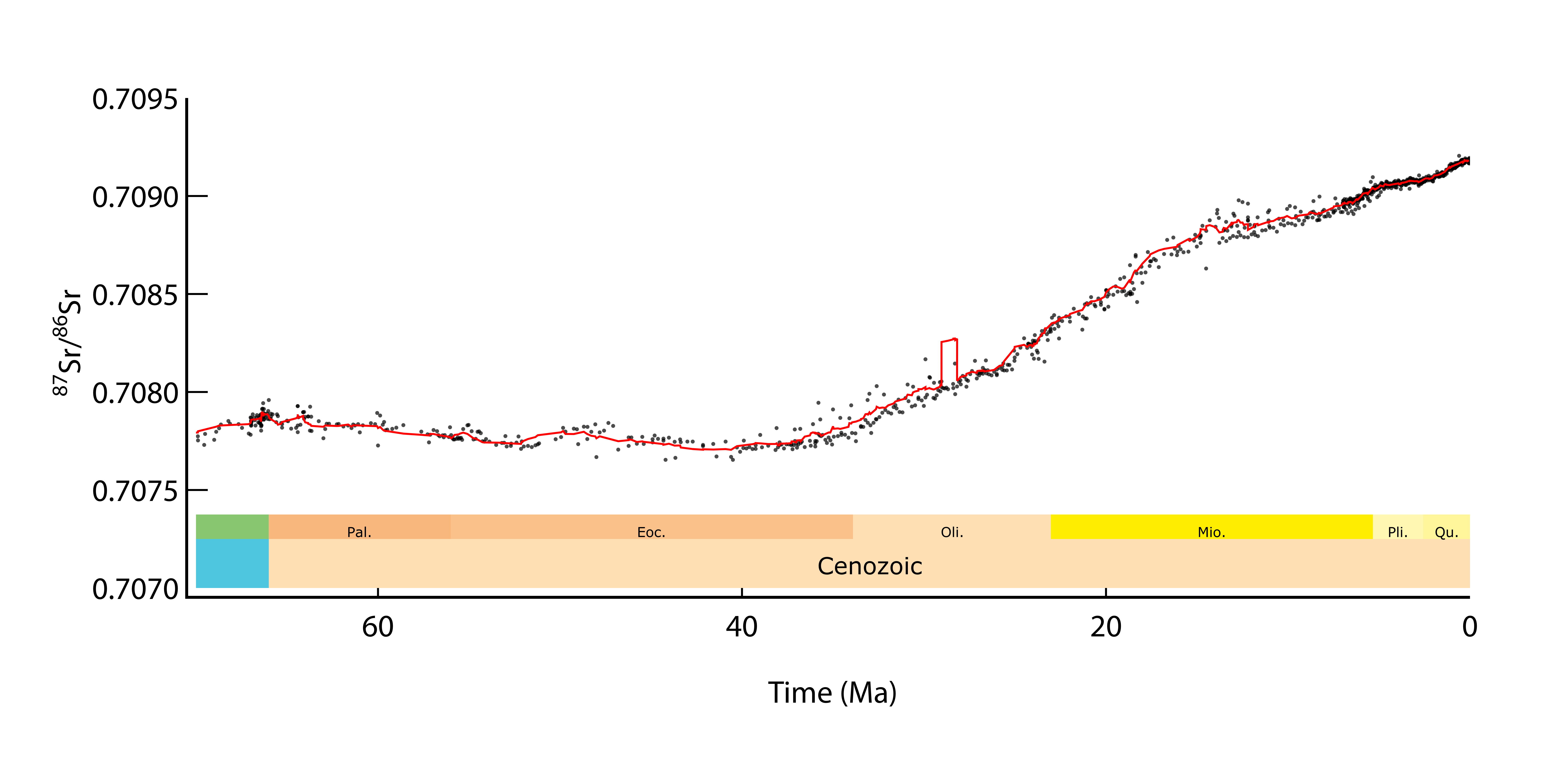
Fig. 3.30 Sr isotopes in marine carbonates over the last 65Ma.

where \(\tau\) is the residence time, \(\sf N_{sw}\) is the total mass of an element in seawater, and \(\sf J_{out}\) is the removal flux of Sr from seawater (into marine carbonates). Sr has a long residence time, of several million years, much greater than the mixing time of the oceans (ca. 100 years). This means that both the concentration and isotope ratio of Sr is constant in seawater, no matter where the water is sampled. This also means that the Sr isotope budget of seawater through time can be conceptualised as a 1-box model:

(3.13)\[\frac{dN}{dt}=\sum(Flux_{in}-Flux_{out})\]

and

(3.14)\[\frac{d(^{87}Sr/^{86}Sr_{sw})}{dt}=\frac{\sum_i\left(\frac{^{87}Sr}{^{86}Sr}\right)_i \cdot(Flux^i_{in}-Flux^i_{out})}{N_{sw}}\]

Sr isotopes in marine carbonates over both the Phanerozoic and the Cenozoic show one of the most elegant geochemical records. Presumably they demonstrate a tectonic control on seawater chemistry over time, and hence Earth’s environment.

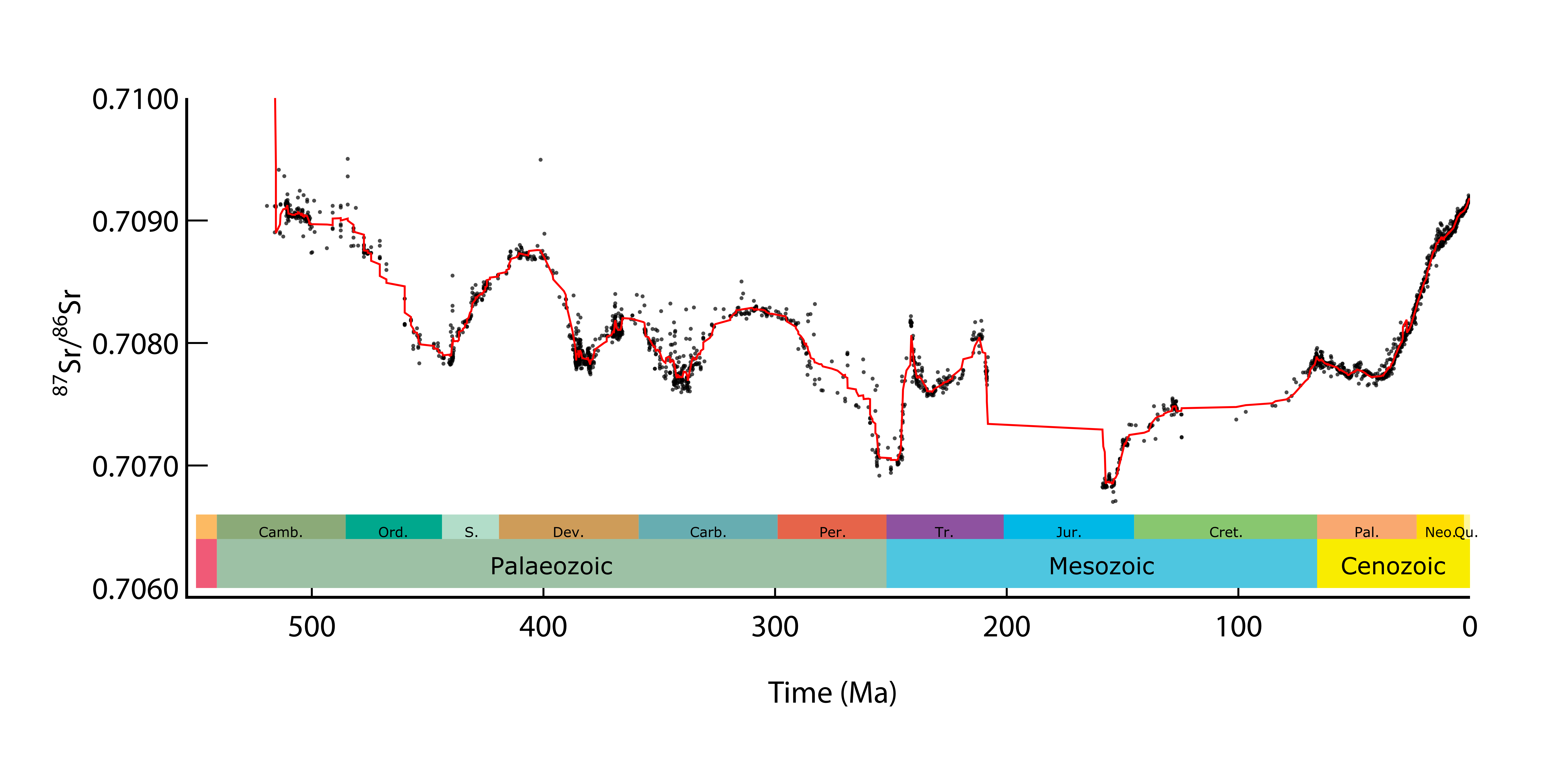
Fig. 3.31 Sr isotopes in marine carbonates over the last 550Ma.

The increase in the \(\sf \frac{^{87}Sr}{^{86}Sr}\) ratio during the Cenozoic (from about 45Ma onwards) is coincident with the collision of India with Asia and the rise of the Himalaya Fig. 3.30. It is widely thought that the variation in the \(\sf \frac{^{87}Sr}{^{86}Sr}\) ratio over time reflects tectonics and mountain building events, driving chemical dissolution and influencing the composition of the hydrosphere and atmosphere.

Radiogenic Osmium isotopes as a tracer of petrogenic organic carbon oxidation

Other tracers of the long term carbon cycle have emerged in the last 20 years, such as the radiogenic osmium (Os) isotope system. \(\sf ^{187}Re\Rightarrow^{187}Os\) with a long half life of 41.6 Ga. Osmium is extremely dilute in natural waters, but is present as \(\sf ^{187}Re\), and as such have a low \(\sf \frac{^{187}Os}{^{188}Os}\) isotope ratio. Organic rich rocks and sulfide minerals (common in organic rich rocks) are enriched in \(\sf ^{187}Re\) and as such have a high \(\sf \frac{^{187}Os}{^{188}Os}\) isotope ratio. There is therefore optimism that the \(\sf \frac{^{187}Os}{^{188}Os}\) isotope ratio may be used to trace the amount of petrogenic organic carbon oxidation over geological time. Interestingly there is a notable increase in the marine record of the \(\sf \frac{^{187}Os}{^{188}Os}\) isotope ratio over the last 35Myr. Is this related to organic carbon oxidation associated with the rise of the Himalaya?

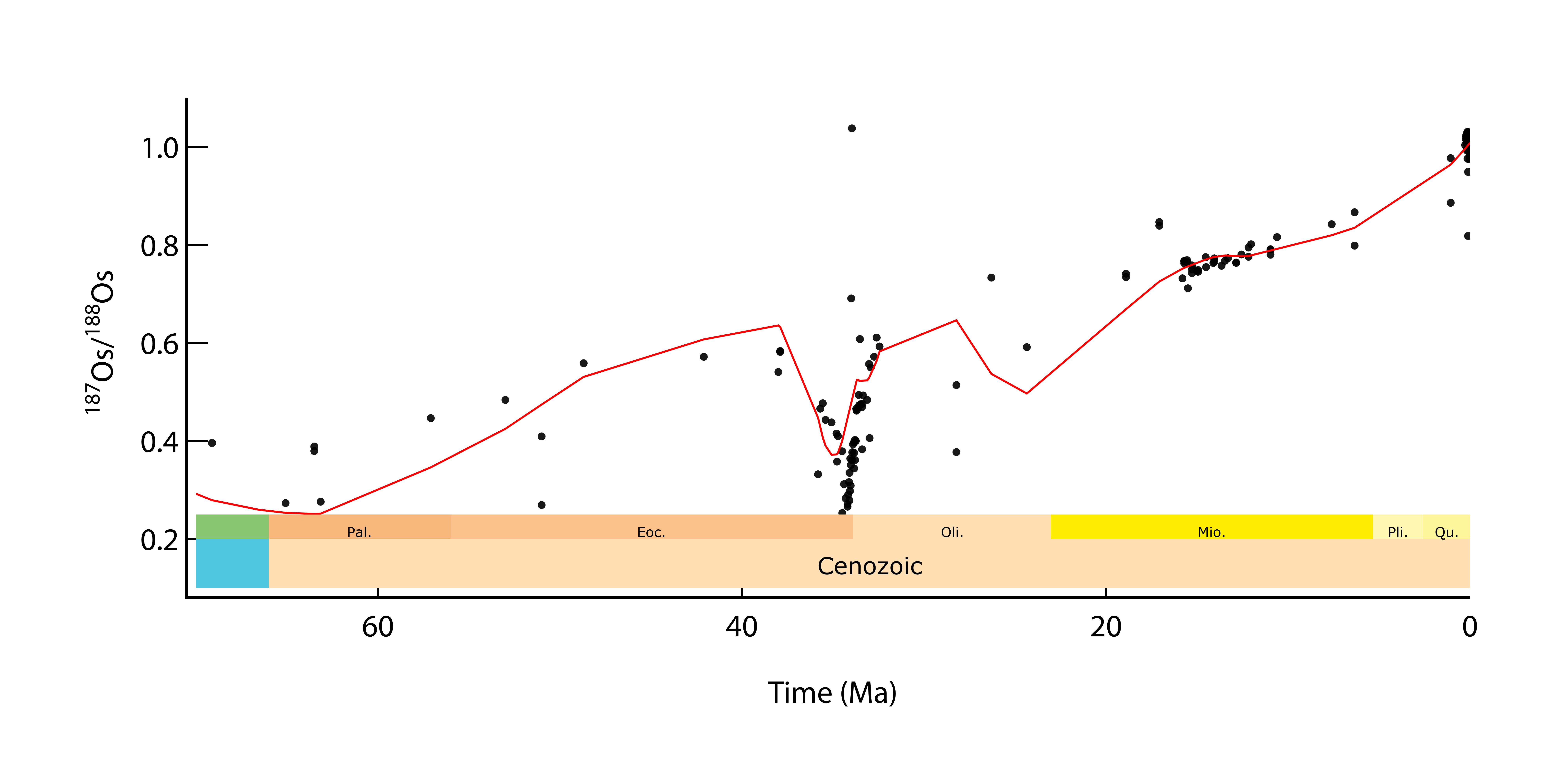
Fig. 3.32 Os isotopes in marine carbonates over time.

The future

Many new records of weathering are emerging, in particular with isotopic tracers. There is a lot still to learn. Stable lithium isotopes are a very good example. What about other planets? Records of weathering having now been discovered on Mars? How did the dissolution of minerals on Mars help shape its hydrosphere?

The emerging view: Can weathering actually release carbon to the ocean-atmosphere system?

Recent work on weathering has considered alternative acidity sources to carbonic acid. Sulfuric acid (\(\sf H_2SO_4\)) is important because if it reacts with carbonate rocks, then \(\sf CO_2\) will be released back to the atmosphere, partially offsetting the \(\sf CO_2\) consumed via carbonate and silicate weathering (3.15) and (3.16). These two reactions release carbon from rocks via two different pathways. (3.15) degasses \(\sf CO_2\) directly to the atmosphere. (3.16) converts carbonate to the bicarbonate ion. The resulting effect on the carbon cycle then depends how how the \(\sf Ca^{2+}\), \(\sf HCO_3^-\) and \(\sf SO_4^{2-}\) recombine at a subsequent time.

Carbonate weathering with sulfuric acid: Carbon source

(3.15)\[\sf H_2SO_4+CaCO_3 \Rightarrow Ca^{2+} +CO_2 +SO_4^{2-}\]

(3.16)\[ \sf H_2SO_4+2CaCO_3 \Rightarrow 2Ca^{2+} +2HCO_3^- +SO_4^{2-}\]

In some large catchments, such as the Peel River (Canada), it is now thought that more \(\sf CO_2\) might actually be released than is consumed via weathering,

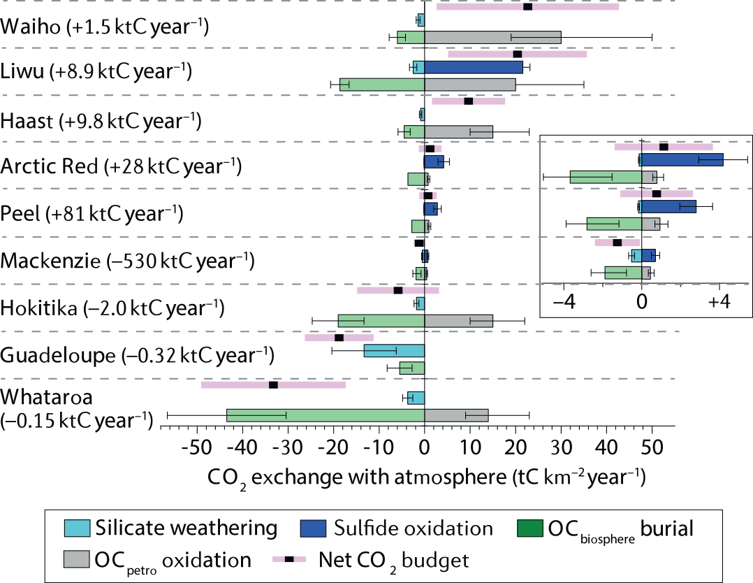
Fig. 3.33 The emerging net budget of the carbon cycle as new data is collected From Hilton and West 2008