4.8. Fundamentals of Aqueous Geochemistry I#
Professor: Nick Tosca (Department of Earth Sciences)
Learning objectives:
Become familiar with basic thermodynamic relationships used to describe the equilibrium state of natural aqueous solutions
Introduce the major classes of reactions common in aqueous solutions
The goal of this lecture is to introduce some key principles which we can use to understand and predict the chemistry of natural waters on Earth (and other rocky planetary bodies where water is/was present).
Introduction#
The chemistry of water undergoes drastic changes as it comes in contact with Earth’s surface, and as it traverses a wide range of physical environments found within Earth’s crust.
Chemical reactions between water and gases, reactions between water and minerals, and reactions occurring among cations and anions dissolved in water, are some of the most important types of reactions to consider in evaluating the processes that can dictate the chemistry of natural waters. These chemical reactions are written like any other chemical reaction, but we must remember to be explicit if we are referring to components in the gas phase (usually marked with subscript “(g)”), the aqueous phase (that is, dissolved in water; we usually use the subscript “(aq)” but this is redundant for ions and cations that have formal charges), or the solid phase (usually marked with a subscript “(s)” if we are referring to a generic solid, or with the mineral name if referring to a specific crystalline solid with a particular structure.
Although these lectures introduce chemical principles which may not be familiar to all students, students are encouraged to consult the references cited below for some good introductions to chemical background (i.e., units, terminology, etc.) that should be useful for the rest of this module. I have also added links to relevant sections of the free online textbook General Chemistry by Petrucci et al.
Equilibrium thermodynamics#
Many treatments and discussions of natural water chemistry are based on equilibrium thermodynamics. In other words, we typically calculate what a particular system would look like if complete chemical equilibrium were attained. In natural systems, complete chemical equilibrium is rarely attained, but this approach is useful because (1) it often provides a good approximation to real systems; (2) it indicates the direction in which changes in chemistry can (or should) take place; (3) it is the basis for the calculation of the rates of natural processes because these depend on how close to, or far from, equilibrium the system may be.
A system at equilibrium is characterised by being in a state of minimum energy. A system not at equilibrium can move toward equilibrium by releasing energy. For systems at constant temperature (T) and pressure (P), which are the ones we’ll deal with the most, the appropriate measure of energy is Gibbs free energy (G).
At constant T and P, Gibbs free energy is related to enthalpy (the heat transferred, H) and entropy (related to disorder, but technically the partitioning of energy across available configurational, vibrational, and electronic states) by:
It is impossible to determine the total amount of G or H a substance possesses in a given state (though we can for S, but dont have time to get into the details); we can only observe and measure changes. Thus, for a chemical reaction such as A + B –> C, the change in energy between the products and the reactants is expressed as:
The sign of \(\Delta G\) for a reaction gives us information about the direction it will proceed. If \(\Delta G\) is negative, the reaction will proceed from left to right as written; if positive, it will proceed from right to left. If the system is at equilibrium, then \(\Delta G = 0\).
Thus, the above equations also imply that at constant T and P, Gibbs free energy can change through the balance between enthalpy and entropy changes.
As a final point, because we can only observe changes in G (or H) as a chemical reaction proceeds, in order to apply real numerical values to these principles, we need to choose a reference reaction. That reference reaction is called the formation from the elements reaction (denoted \(\Delta G_{f}^{o}\) or \(\Delta H_{f}^{o}\)) and is written as a balanced chemical reaction for the formation of any substance from the elements in their stable states at standard temperature and pressure (commonly 298K and 1 bar). The reason for this choice is that if our reaction of interest is written in terms of these reactions, then all of the elements cancel and \(\Delta G_{r}\) for our reaction is expressed in terms of the differences between the formation values for the substances appearing in our reaction of interest.
As an example of how this works, consider the standard Gibbs free energy of formation from the elements (\(\Delta G_{f}^{o}\)) for the minerals calcite and aragonite (both have the fomula CaCO\(_{3}\) but have different crystalline structures):
Lets say we are interested in the Gibbs free energy change of the reaction where calcite converts to aragonite. To obtain this reaction, we would add the two reactions above together (but reversing the first one). Doing so would result in cancellation of all of the elements in their stable states (the same is true for any balanced chemical reaction). Thus the total Gibbs free energy change of the reaction can be generalised to:
For reactions occurring in natural waters, we often deal with reactions that involve a change in composition, and so we must come up with a way to assess how each individual species affects the free energy of the system. Consider the reaction describing the conversion of the mineral calcite to the mineral dolomite in aqueous solution:
We may wish to know at what Mg\(^{2+}\) and Ca\(^{2+}\) concentrations this reaction is at equilibrium.
To do this, we use the chemical potential (\(\mu\)), which can be thought of as the amount of G per mole of a substance. For some substance (ion, gas, compound, etc.) i:
where n is the number of moles of component i being added to the system. This means that at constant T and P, the change in Gibbs free energy of our system will be determined by the contributions of the different chemical components present. Thus, at equilibrium, the chemical potentials of all of the components in the system must be the same in each phase (i.e., the chemical potential of Ca in Ca\(^{2+}\) must be the same as in CaMg(CO\(_{3})_{2}\)).
In order to use these principles in practice, two final and related quantities are required. The first is fugacity, which can be thought of as an effective pressure, which is commonly used in connection with gases. The second is activity, which can be thought of as an effective concentration, which is used in connection with liquid and solid phases. These are defined by:
where \(\mu_{i}^{o}\) refers to the chemical potential of component i in its standard state, R is the gas constant (8.314 J/mol K) and T is temperature in kelvin.
The standard state is simply an arbitrary point of reference chosen to make solving a particular problem easier rather than any theoretical consideration. For natural waters, the standard states in use dictate that the activity of a component approaches its molar concentration as its concentration decreases. This leaves one more parameter to define, which is the activity coefficient, which expresses the difference between activity and molar concentration:
thus, \(\gamma_{i}\) approaches 1 as \(m_{i}\) approaches 0.
The equilibrium constant
We have a parameter, the activity, that captures the influence of system constituents on Gibbs free energy, but how do we actually use this in practice? Consider a general chemical reaction of the type:
where \(a\), \(b\), and \(c\) are stoichiometric coefficients, \(A\) and \(B\) are the reactants, and \(C\) is the product. For each constituent in the reaction, we have the molar amounts of Gibbs free energy (or chemical potentials):
We can determine the change in chemical potential (that is, the Gibbs free energy per mole) by subtracting the reactants from the products. So for our general reaction we have:
Written in a more general way:
where \(\nu_{i}\) is the stoichiometric coefficient. The \(\prod_{i}\;a_{i}^{\nu_{i}}\) term is given the symbol \(Q\), so that:
At stable equilibrium, the activities assume a special meaning, and the activity term is given the symbol \(K\). This is different from \(Q\) which is the same term mathematically, but the activities can assume any value, which means that the system is not necessarily at equilibrium:
or
Remembering that \(\Delta \mu_{r}^{o}\) is simply the standard state Gibbs free energy change (expressed in terms of moles per component in the reaction), this equation is more often written as:
This equation is often called the most useful equation in thermodynamics. Its important to note that \(K\) (the equilibrium constant) is a constant for a given system at a given temperature (or pressure and temperature) and is called the equilibrium constant. This is useful because with a few standard state free energies, we can calculate an almost indefinite number of equilibrium constants. This gives us critical information about a vast range of reactions. We will go through some specific examples in the lecture, and for the rest of the notes for this lecture, we’ll see how to apply this to the main types of reactions that occur in aqueous systems.
Chemical reactions in aqueous solutions#
Liquid water and hydrogen bonding
Liquid water has several unusual and even unique physical properties (i.e., heat capacity, heat conduction, heat of vaporisation and fusion, dielectric constant, etc.) that mainly reflect the fact that water molecules do not behave independently; they are attracted to each other and many solutes by moderately strong “hydrogen bonds”.
Hydrogen bonding is a consequence of the molecular structure of water. Oxygen’s four remaining valence electrons (those not tied up in forming the two O-H bonds) occupy two orbitals opposite the hydrogen atoms in a distorted cube arrangement. This leads to a dipole moment, or partial charge located on either end of the H\(_{2}\)O molecule. These electron pairs interact with hydrogen atoms of adjacent water molecules to form hydrogen bonds.
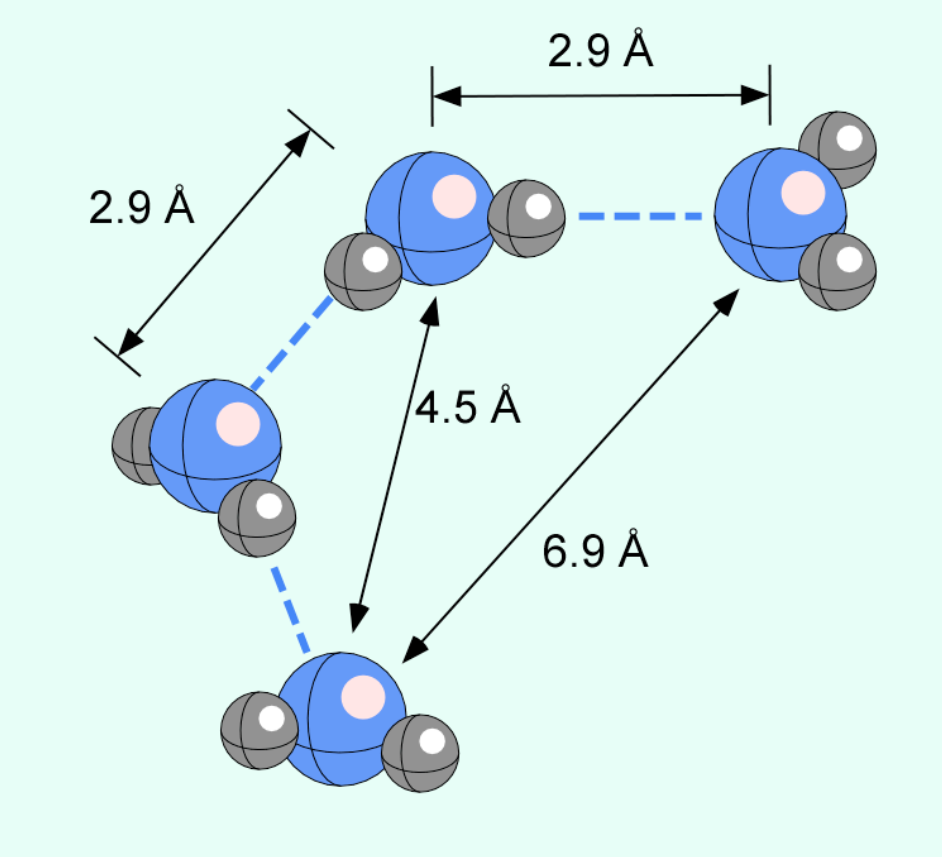
Fig. 4.67 Schematic diagram showing some common geometries and distances across which neighbouring H\(_{2}\)O molecules interact through hydrogen bonding.#
Ion hydration and hydrolysis
The dipole moment of water molecules means they are attracted to ions in solution, which is why ionic compounds readily dissolve in water.
In general, the higher ionic potential (that is, the formal charge of the ion divided by the ionic radius), the more strongly bound water molecules are in the first “shell” of H\(_{2}\)O molecules surrounding the ion. Both increasing charge (for a given ionic radius) or decreasing radius (for a given charge) means that water molecules are bound more strongly to the ion.
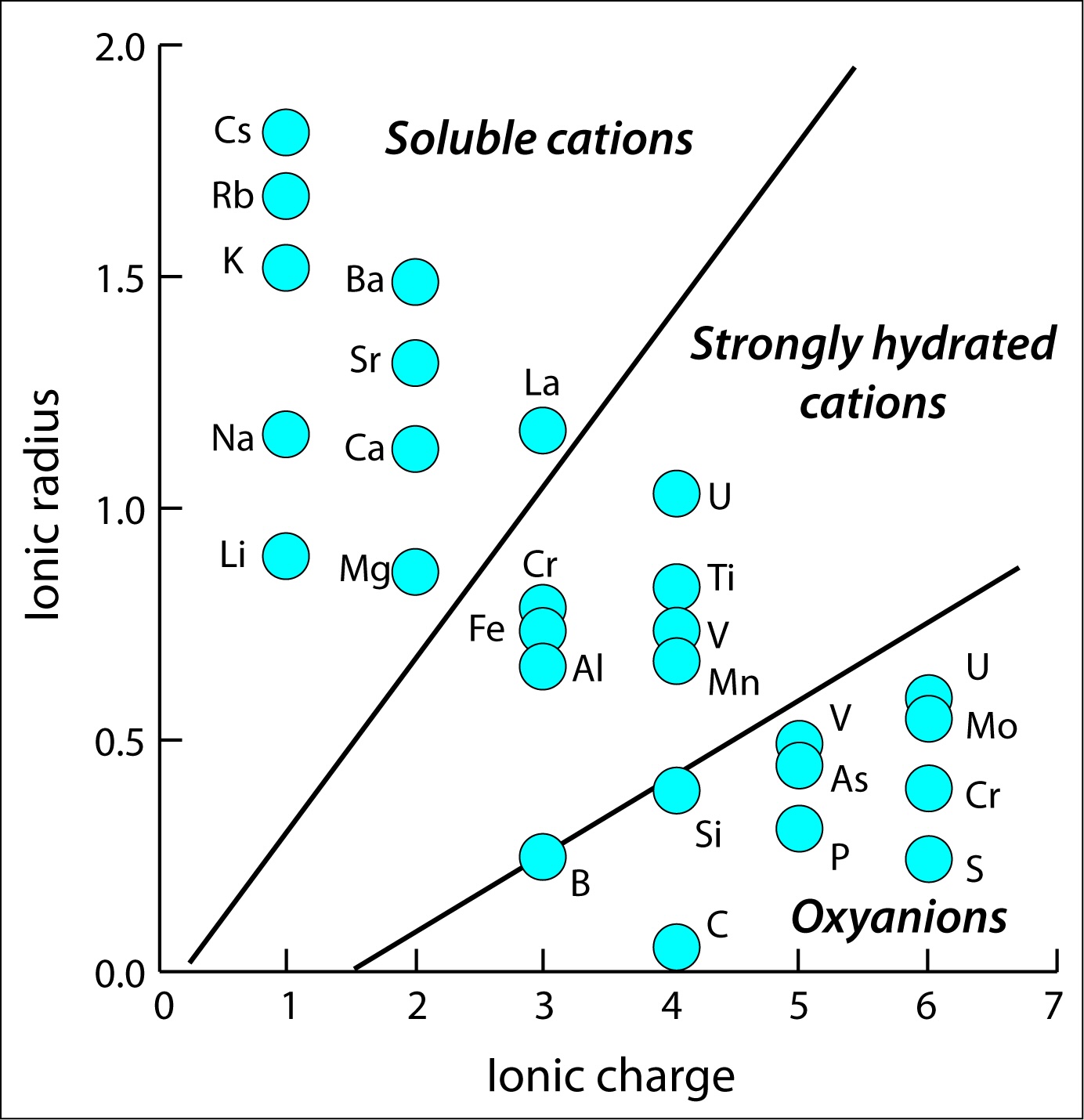
Fig. 4.68 Plot of the ionic radius for various ions in aqueous solution as a function of their formal ionic charge. As the charge to radius ratio increases (increasing ionic potential), the most stable congifuation results in the formation of oxyanions such as CO\(_{3}^{2-}\) for the C\(^{4+}\) cation, and H\(_{4}\)Si\(_{4}^{o}\) for the Si\(^{4+}\) cation.#
If ionic potential is high enough, then the addition of a H\(_{2}\)O molecule during ion hydration can be accompanied by the loss of a proton (H\(^+\)). This is referred to as a hydrolysis reaction; these reactions dictate the solubility of metal ions in water and are sensitive to pH. A good example is the first hydrolysis reaction of Fe\(^{3+}\):
Hydrolysis reactions such as these typically happen in consecutive steps and are promoted by increases in pH.
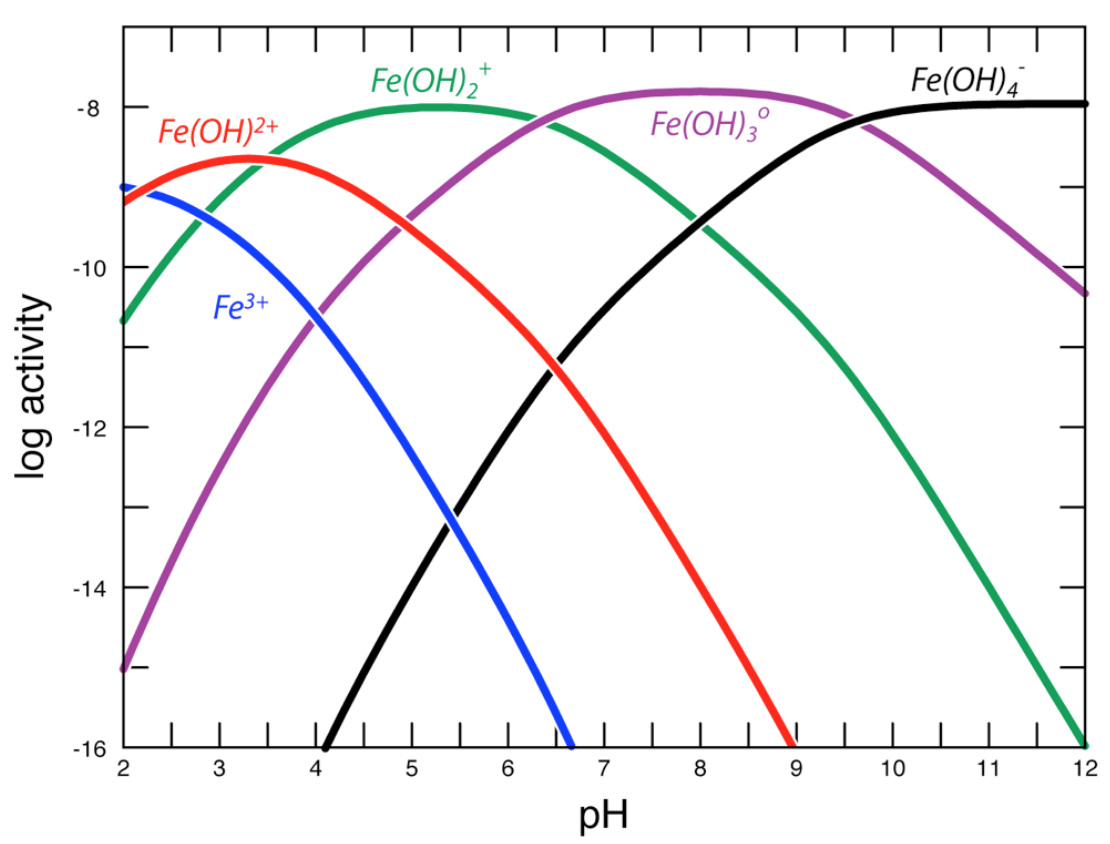
Fig. 4.69 Plot of the logarithm of the activities (or effective concentrations) of aqueous species formed through successive hydrolysis reactions with the aqueous Fe\(^{3+}\) ion. With increasing Fe concentration, the highly hydrated complexes combine to form clusters which then serve as the first step in the precipitation of Fe-hydroxide and Fe-oxide minerals from solution.#
Ion pairing and complexation
Another important class of reactions occurring in natural waters involves the combination of positively charged ions (cations) with negatively charged ions (anions) to form a complex in solution. Consider for example:
where the superscript “o” denotes a neutrally-charged complex dissolved in solution.
The relationship between the equilibrium constant (see above) for this reaction and the ion activities can be written using the law of mass action, a definition which arises from the derivation above:
The relatively large value of K at equilibrium tells us that the product is strongly favoured when the reaction is at equilibrium.
Ion pairing or complexation reactions are important because they can reduce the concentration of free ions, increase the solubilities of minerals, they can stabilise dissolved species, and they can change the reactivity of aqueous components.
Acid-base reactions
Acid-base reactions are a fundamental aspect of natural waters. These involve the loss or gain of protons as in the following example:
Applying the law of mass action to this reaction allows us to express the activities in terms of the equilibrium constant for the acid dissociation reaction (for a generic acid HA):
We can use the \(p\) function to take the natural log of the acid dissociation constant:
This also leads to the definition of pH, which is:
Because at equilibrium the activities of A- and HA are usually close in value, a common approximation is that \(pK_{a} \approx -\log a_{H+} = pH\). This gives us an indication of how strong the acid is. Strong acids have low \(pK_{a}\) values and weak acids have higher values. In other words, the \(pK_{a}\) for HCl is -6.3, which means that the activities of Cl- and HClo are equal at a pH of -6.3. Compare this to acetic acid, for which the \(pK_{a}\) is 4.76.
Activity-concentration relationships in aqueous solutions
How do we relate measurable molar concentrations of ions to their activities so we can perform thermodynamic calculations?As we discussed above, the activity coefficient can be viewed as a “correction factor” encompassing the departure from the ideal standard state. Generally, for aqueous solutes, the departure from ideal behaviour becomes greater as solute concentrations increase. This is because non-ideal behaviour originates from long-range electrostatic interactions between ions (at low concentrations), giving way to short-range interactions between multiple ions at higher concentrations. This can become complicated for natural waters. Imagine, for instance, we are interested in determining the activity coefficient for Ca\(^{2+}\) and CO\(_{3}^{2-}\) in an evaporated brine derived from seawater. Even if we are dealing with a generally low concentration of Ca\(^{2+}\) and CO\(_{3}^{2-}\), the Na\(^{+}\) and Cl\(^{-}\) concentrations could be enormous. All of these solutes (e.g., Na, Cl, Ca, CO\(_{3}\)) would thus be behaving non-ideally.
To deal with this complexity, we first need a way to express how concentrated a given multi-component solution is. For aqueous solutions, that turns out to be the ionic strength:
where \(z_{i}\) is the charge of ion \(i\) and \(m_{i}\) is its molality (moles of component per kg solvent).
It turns out that natural aqueous fluids exhibit an enormous range in ionic strength spanning several orders of magnitude from very dilute meteoric water to highly concentrated brines. The ionic strength is a master variable which is required in all of the available models for calculating ion activity coefficients (and therefore activities). In general, these models each are appropriate over different ranges in ionic strength, and this (along with temperature/pressure considerations) is the general means of deciding which model is most appropriate. It is not critical to remember the details of the models at this point because they are generally empirical in nature.
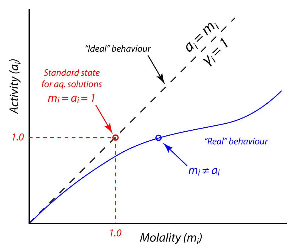
Fig. 4.70 Schematic showing the relationship between activity (or the effective concentration) of a constituent i, and its molar concentration (in molality, or moles/kg solvent). As concentrations decrease, activity and concentration converge to the same value (as the activity coefficient, \(\gamma_{i}\) approaches 1). At high concentrations, non-ideal behaviour (resulting from interaction between neighbouring cations and anions in solution) results in significant deviations between activity and concentration, resulting in \(\gamma_{i}\) that deviate from unity (and require empirical estimation). The “standard state”, or reference state for aqueous solutions, chosen for mathematical convenience, is a hypothetical solution where a 1 molal solution of component i has an activity equal to 1.#
Further reading#
Anderson, G.M. Thermodynamics of natural systems, 3rd edition. Cambridge University Press (2017).
Brezonik, P.L. and Arnold, W.A. Water Chemistry, Oxford University Press, 782p. (2011)
Stumm, W. and Morgan J.J., Aquatic Chemistry, Wiley Interscience, 1022p. (1996)