Venus II: Venus Over Time

3.12. Venus II: Venus Over Time#

Learning Objectives:

This course is about Venus in the past and as an exoplanet. It will cover:

Connection between Venus today and Venus in the past.

Different proposed pasts for Venus: always hot, runaway greenhouse, recently habitable.

Connections between Venus and exoplanets: Climate + Photochemistry

Brief Overview of Atmospheric Evolution#

Box Model#

When we think about Venus over time, most of what we will be talking about is the atmospheric evolution of Venus. Before we look into the atmospheric evolution of Venus, let’s consider the evolution of atmospheres in general.

The simplest picture of atmospheric evolution takes a box model, where the entire atmosphere is treated as a box where we can put molecular species, and remove them. This is a reasonably good approximation when the molecular species are stable, so they don’t change too much throughout the atmosphere. To figure out if this is a decent approximation for a given species, \(i\), just take the surface mixing ratio of the species, \(f_i\), multiplied by the gas density, \(n\) (cm\(^{-3}\)) and the scale height of the atmosphere:

(3.24)#\[H_0 = \dfrac{kT}{\mu_{\rm av} m_p g},\]

where \(k = 1.38 \times 10^{-23}\) J/K is Boltzmann’s constant, \(T\) (K) is the temperature at a given atmospheric height, in our case, the surface. \(\mu_{\rm av}\)is the average mass of the atmosphere in units of proton masses, \(m_p = 1.673 \times 10^{-27}\) kg is the mass of a proton, and \(g\) (m s\(^{-2}\)) is the gravitational acceleration at a given atmospheric height, again, in our case, the surface. If this value deviates considerably from the total column density,

(3.25)#\[N_i = \int_{0}^{\infty} n_i(z) \; dz,\]

then the box model is a bad approximation for species \(i\) to the degree of deviation, \(\epsilon\):

(3.26)#\[n_i H_0 = N_i \pm \epsilon N_i\]

Let’s assume the deviation is small. How does the box model work? Again, picture a box, with molecular species going in, and going out. We need fluxes into and out of the box. Those fluxes, represented as \(\Phi\) (cm\(^{-2}\) s\(^{-1}\)) can represent fluxes from oceans or lakes, due to evaporation, or release of molecules from some surface chemistry, or outgassing from a volcano. Losses can happen through rain, or dry deposition: the molecular species reacts with something on the surface, maybe it’s being eaten by a microbe, or respirated by a toad. Losses can also happen via escape. We’ll talk about that in a bit more detail later. You can see the figure below for a picture of these different fluxes coming in and going out of the atmosphere.

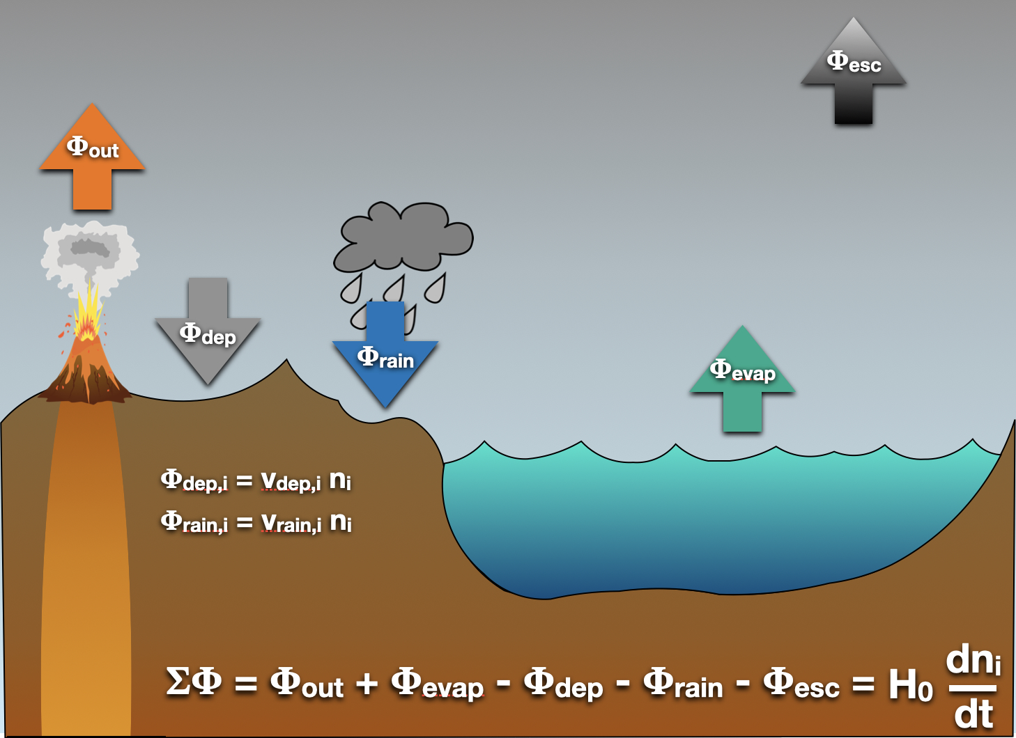
../../_images/venus-evolution.jpg — Fig. 3.86 **Atmospheric Sources and Sinks.** Here we take into account various sources and sinks for the atmosphere. We have a bunch of fluxes, \(\Phi\), all with units of cm\(^{-2}\) s\(^{-1}\). There’s the sources: outgassing (\(\Phi_{\rm out}\)), evaporation (\(\Phi_{\rm evap}\)). And the sinks: rainout, or wet deposition (\(\Phi_{\rm rain}\)); dry deposition (\(\Phi_{\rm dep}\)); and escape (\(\Phi_{\rm esc}\)). Of all of these, escape alone involves completely removing something from the system. The rest may count as effective removal, but are thought to leave the global state of the planet unaffected.#

We can use these specific sources and sinks, and write out a differential equation, much like the one that appears on the figure:

(3.27)#\[H_0 \dfrac{dn_i}{dt} = \Phi_{\rm out} + \Phi_{\rm evap} - v_{{\rm rain},i} n_i - v_{{\rm dep},i} n_i - \Phi_{{\rm esc},i}.\]

If I divided both sides by the scale height, this would look equivalent to the chemical kinetics equation from last lecture, except for one term: \(\Phi_{{\rm esc},i}\). We would expect this to be linearly proportional to the number density of the species in the atmosphere, and indeed it (generally) is, but the constant of proportionality depends a great deal on the way the molecular species ends up escaping. Once we know what dominates, we can solve this equation much like we solve any other chemical kinetics equation.

Often, these terms can get pretty big, especially when life is involved. Here “big” means \(\gtrsim 10^{11}\) cm\(^{-2}\) s\(^{-1}\), and if that’s all there was going into an atmosphere like Earth’s, a 1 bar atmosphere of that species would build up in a matter of just a few million years.

But what tends to happen is that sources and sinks more or less balance out for much of Earth’s, and other planetary, history (again, presumably, and for most planets). And so the overall change is very slow. Every once in a while, like very early in Earth’s history, or during its great oxygenation event, things changed very quickly. Sometimes the system is thrown out of balance. Even then, sinks will catch up pretty soon and bring the system back into balance.

Escape#

How do atmospheres escape? They can escape whenever the energy of any individual molecular species exceeds the escape velocity, and when that molecular species is unlikely to bump into anything along the way, scattering it back into the atmosphere. Giant impacts can initiate escape. Solar flares could as well. But just the temperature of a gas can lead the gas to escape. Especially the lighter part of the atmosphere, like hydrogen, can escape when it reaches the exobase, the part of the atmosphere where the scale height is about the same as the length scale for a collison:

(3.28)#\[\dfrac{kT_{\rm exo}}{\mu_{\rm av, exo} m_p g_{\rm exo}} = \dfrac{1}{\sigma \, n_{\rm exo}},\]

where exo added to everything means, what that variable is at this exobase, and \(\sigma\) (cm\(^2\)) is the average collisional cross-section: if I kept choosing two molecular species at the exobase at random, figured out their cross-sections, and found that average, that’d be the average collisional cross-section.

The above equation can be solved to figure out what the height of the exobase is (\(r_{\rm exo}\)). Then it’s just a matter of figuring out what fraction of a Maxwell-Boltzmann distribution of particle velocities are above the escape velocity, for a given species, \(i\). We’ll work this out on the board, and the answer is:

(3.29)#\[\Phi_{{\rm esc},i} = \dfrac{n_{{\rm exo},i}v_{x,i}}{\sqrt{4\pi}}\Big(1 + \lambda_{Ji}\Big)e^{-\lambda_{Ji}},\]

where \(v_x = [2kT/(\mu_i m_p)]^{1/2}\) is the expectation Boltzmannian velocity for species \(i\), where \(\mu_i\) is the mass of that species in proton masses. And \(\lambda_{Ji}\) is the Jeans escape parameter for species \(i\):

(3.30)#\[\lambda_{Ji} = \dfrac{GM_pm_i}{kTr_{\rm exo}},\]

where \(M_p\) (kg) is the mass of the planet, and \(G = 6.674 \times 10^{-11}\) N m\(^2\) kg\(^{-2}\) is the gravitational constant.

If this escape mechanism dominates, or if some other excape mechanism matters more, and the escape of light atoms and molecules is very fast, then it can turn out that light species escape faster than they can be restored to hydrostatic equilibrium. In this case, a chunk of the atmosphere above a certain height will be lost, and the rate at which it can be restored is the fastest possible rate at which that molecular species can be lost, so long as it needs to diffuse through the rest of the atmosphere to escape. Some escape mechanisms, particularly from giant impacts, can overcome this limitation. But when this limitation is approached, the concentration of that constituent above the homopause (where all the atmosphere is well-mixed) deviates from hydrostatic equilibrium. See the below figure.

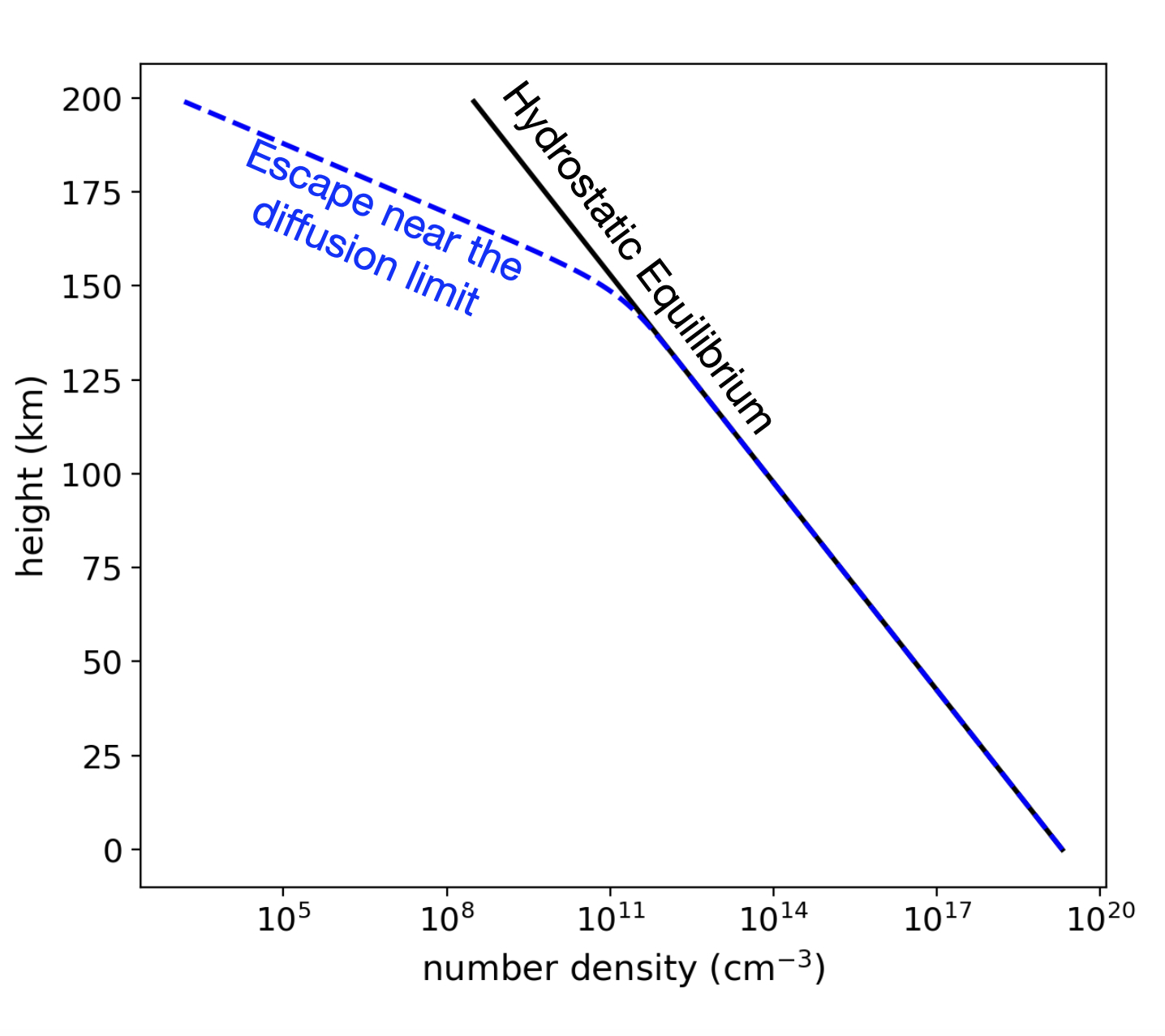
../../_images/diffusion-limit.jpg — Fig. 3.87 **Diffusion-Limited Escape**: Some light constituent of the atmosphere deviates from the expected hydrostatic equilibrium profile, because so much of it is escaping, and it’s escaping faster than diffusion can replace it.#

This limitation is called the Diffusion Limit. We will show in class that, given this limit:

(3.31)#\[\Phi_{\rm esc} \leq \dfrac{D_i}{H_0} \, n_i,\]

where \(D_i\) (cm\(^2\) s\(^{-1}\)) is the diffusion coefficient for species \(i\) diffusing past the average atmospheric constituent.

If you have trouble following these derivations, or want to dig into greater detail, I recommend looking at Chapter 5 of Catling & Kasting’s “Atmospheric Evolution of Inhabited and Lifeless Worlds” (Catling & Kasting 2017).

Atmospheric Redox (Im)Balance#

An atmosphere where nothing condenses out, nothing escapes, nothing enters or leaves, will keep perfect mass balance. Even if we allow all kinds of crazy chemistry reactions, none of those will significantly change mass balance. So long as the atmosphere is made up of stable radioisotopes, this also means that the numbers of different atoms will remain constant over time. The same is true if the box model equation equals zero for every species.

But most atmospheres have some molecular species that will condense out, and others will be absorbed into those droplets and rain out, and all of the sudden, we lose mass balance. We could try to track the atmosphere by its change of mass, but this will be a big mess. On a warmer day, there’s more water vapor in the air, and carbon dioxide is breathed in and out by most species right now, and is at a low enough abundance that it can change considerably. Sulfur dioxide is belched out of volcanoes, and then turns into sulfuric acid in rain drops and is removed again.

There is a powerful concept for bookkeeping called atmospheric redox. Redox means something specific in chemistry, that we will learn more about in C3. But atmospheric redox means something a little different, very useful for tracking important long-term changes in an atmosphere.

Here what we do is we define redox by setting certain values for oxygen, and values of opposite sign for hydrogen. We can set these values as we like, and can also choose what molecules have the value of zero. If we choose wisely, we can keep track of changes in the atmosphere that involve more oxygens (e.g. O\(_2\)) or hydrogens (e.g. CH\(_4\)), while zeroing out species that change a great deal over very short timescales (like water and CO\(_2\)). These changes are chemically important, for reasons that will be chemically clearer after C3. For now, it’s useful to see that life tends to remove molecules or add molecules to the atmosphere that have an effect on the overall redox balance, and also that H\(_2\) and H tend to escape very easily from the atmosphere of Earth and other planets of similar mass, so it is good to track the hydrogen in particular.

We will keep with the convention of Catling & Kasting, for ease of translation, but we can choose any values and zeros we like, so long as they are stoichiometrically consistent. We will set H\(_2\) = +1 and H\(_2\)O = 0. This decision forces us to choose O\(_2\) = -2, because:

(3.32)#\[\begin{split}\begin{split} 2 {\rm H_2} + {\rm O_2} &\rightarrow 2 {\rm H_2O} \\ 2 \, (+1) + x = 0 \\ x = -2 \end{split}\end{split}\]

Using this same technique, we can find out that, if we define CO\(_2\) = 0, CO carries the same reducing power as H\(_2\), using the same chemistry we already discussed for the CO\(_2\) stability on Mars.

(3.33)#\[\begin{split}\begin{split} {\rm H_2O} + h\nu & \rightarrow {\rm OH} + {\rm H} \\ {\rm CO} + {\rm OH} & \rightarrow {\rm CO_2} + {\rm H} \\ {\rm H} + {\rm H} + {\rm M} & \rightarrow {\rm H_2} + {\rm M} \end{split}\end{split}\]

If we sum this equation, we get:

(3.34)#\[\begin{split}\begin{split} {\rm H_2O} + {\rm CO} &\rightarrow {\rm H_2} + {\rm CO_2} \\ 0 + x = +1 + 0 \\ x = +1 \end{split}\end{split}\]

Here we start to see the power of this bookkeeping technique: its universality. No matter how CO\(_2\) is restored in the atmosphere of Venus, it will involve adding the equivalent of a single H\(_2\) to the atmosphere, though of course that equivalent need not be H\(_2\) itself. If there’s a liquid water ocean, and photochemistry is important, then the H\(_2\) equivalent will almost always end up being H\(_2\) itself.

I suggest you use these techniques to figure out the redox values of CH\(_4\) and, defining N\(_2\) however you like, find the redox value of HCN. You can consult Catling & Kasting (2017), their Chapters 7 and 8, for more details.

For many planets H\(_2\) escapes the atmosphere preferentally. The atmospheres of those planets will slowly become more oxidized. It’s important to keep in mind that this redox evolution does not happen in a vacuum. It happens in an atmosphere in contact with a surface, maybe an ocean, at least some rocks or something. If the atmosphere becomes too reducing, it will begin to change the chemistry on the surface, and the sub-surface, over timescales set by the motion of molecules on the surface and beneath. As the surface becomes more reducing, this will, at least temporarily, remove that reducing power from the atmosphere. The same thing if H\(_2\) keeps escaping, the oxygen will itself become removed in the ocean, to form oceans of hydrogen peroxide, and in rocks, to form rocks with very oxidized iron and other metals. See Harman et al. (2015).

It is also worth mentioning that this bookkeeping method is just that. A way of keeping track of something that is presumably of interest. Our bookkeeping is designed right now to be very sensitive to H\(_2\), which can easily escape. Our focus, and the way we set up our bookkeeping might change if our understanding of H\(_2\) escape changes. For example, even a relatively small change in the H\(_2\)O photoabsorption cross-section, can affect the fate of H\(_2\), whether it escapes, or whether it ends up reacting with carbon-bearing molecules in the atmosphere and forming organics, like formaldehyde (HCHO) that rain out. See Ranjan et al. (2020). If most of the H\(_2\) equivalents rain out, this becomes a less convenient bookkeeping convention!

Three Histories of Venus#

Venus today is dry and devoid of life, at least for life as we know it. Was it always this way? Over the years, there have been three different trajectories proposed for Venus’s past, that are broadly consistent with present-day Venus, but each of which contains some unsolved mysteries.

Trajectory 1: Maybe Venus never had much water. Either the water never condensed, and escaped very early on, or not much water ever got to Venus for some reason. Mystery: The D/H ratio is very high on Venus, compared to protosolar nebula, or Earth, or really any other environment. For the protosolar nebula, D/H \(\sim 2 \times 10^{-5}\). For the Earth and most other interplanetary rocky objects, D/H is between 1 and 5 \(\times 10^{-4}\). For Venus’s atmosphere, it’s about 1.5%! Escape can explain this difference. Just carry out the derivation for deuterated hydrogen instead of H\(_2\) above, and see how different the escape rates are. You can predict the D/H using escape of hydrogen, but not if there was no hydrogen, no water, really to start with. So if not escape, what explains Venus’s D/H ratio?

Trajectory 2: Maybe Venus had a lot of water, but lost it very early on. This is effectively the scenario proposed by Turbet et al. (2021), though their scenario would also be consistent with our Trajectory 1. Venus quickly underwent a greenhouse runaway, due to its proximity to the Sun, and enhanced by the formation of clouds preferentially on the night side, allowing the sunlight to get deep into the atmosphere and then trapping the heat on the night side. Mystery: If Venus lost so much of its H\(_2\), it lost a lot of reducing power, and the leftover O\(_2\) should have oxidized the surface and atmosphere considerably. But Venus’s atmosphere is, if anything, a bit reducuing. Almost all the constituents of Venus’s atmosphere have a redox value of 0, or slightly positive. OCS has a redox value of +3, and CO of +1, and these are the most abundant constituents of Venus’s atmosphere with a non-zero redox value. What happened to all the oxygen? Where did it go, and what did it oxidize?

Trajectory 3: Maybe Venus was habitable until very recently. Different climate models, proposed by Way et al. (2020), suggest Venus could have been habitable even until today. They use different initial conditions to Turbet et al., and a different model, and they get that clouds preferentially form on the day side. This blocks light from getting absorbed deep in the atmosphere, and leaves all the heat to radiate out on the night side. We know this isn’t the way Venus is today, so something must have happened to cause it to get knocked out of its habitable state. Mystery: What was it that knocked Venus off of its habitable condition? And where did all the water go? Why is Venus so dry, even when considering the water content of its volcanic emissions (see Constantinou et al. 2024)?

Future missions will be needed to sort out which of these is the correct trajectory, if any.

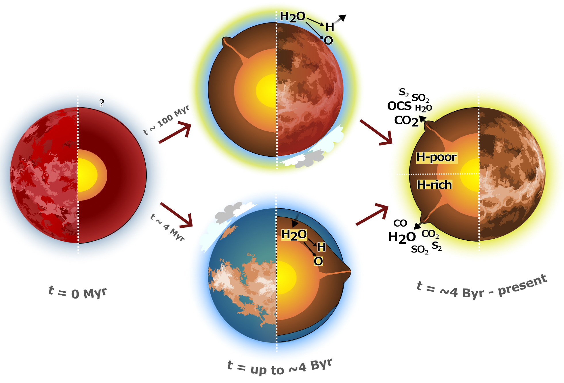
../../_images/three-venus.jpg — Fig. 3.88 **Three Trajectories for Venus**: Either Venus never condensed its water (**Trajectory 1**), or Venus condensed its water for a short time and then lost it to runaway greenhouse (**Trajectory 2**), or Venus kept its water as liquid water, as a stable climate state, until some catastrophic event, e.g. the release of enormous amounts of CO\(_2\) in a global volcanic event, threw Venus into a runaway greenhouse, as little as \(\sim 500\) million years ago (**Trajectory 3**). From Constantinou et al. (2024), their Figure 1.#

Venus as an Exoplanet#

Venus Around Other Stars#

It turns out that when you place Venus around other stars, quite a few of the sulfur-bearing species tend to survive significantly higher up in the atmosphere, including OCS. The cloud heights also change. Jordan et al. (2021) give a lot of the details of this. See the figure below, which shows how OCS and H\(_2\)S survive much more easily for planets around cooler stars.

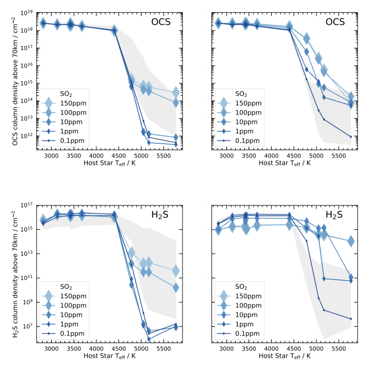
../../_images/ocs-exovenus.jpg — Fig. 3.89 **OCS and H\(_2\)S Survival on Exo-Venus** When Venus is placed around cooler stars, the sulfur species H\(_2\)S and OCS survive at much higher abundances, above the clouds. They may be observable with future telescopes, and would indicate the presence of a Venus-like atmosphere, albiet an atmosphere with different photochemistry, due to its different host star. From Jordan et al. (2021), their Figure 10.#

Could life exist in the clouds of Venus, or other Venus-like exoplanets? Not life like we know it, but some of the most interesting new work in Venus science right now involves taking biomolecules, like nucleobases and amino acids, and placing them in sulfuric acid to see what happens. It turns out most of these molecules survive (Seager et al. 2023, Seager et al. 2024), and some of them can form spherical membranes, that look a bit like cells, shape-wise (Duzdevich et al. 2024). There are also tentative signals of claimed biosignatures such as phosphine and ammonia in Venus’s clouds (Greaves et al. 2021; Mogul et al. 2021; also https://www.theguardian.com/science/article/2024/jul/17/signs-of-two-gases-phosphine-ammonia-in-clouds-of-venus-life ), but sorting those claims out is a whole other story (e.g. Bains et al. 2021).