Exoplanets II: Architectures

2.2. Exoplanets II: Architectures#

Learning objectives:

To understand the diversity of exoplanetary system architectures

To understand the biases inherent to our exoplanetary catalogue and key features suchas the radius valley

To be aware of language used to characterise exoplanetary systems, such as the habitable zone, or resonant chains

This lecture will discuss how unveiling the population of exoplanets has contradicted our view of what a typical planetary system might look like and how are perspective is still biased by the limitations in current detection methods for exoplanets.

Planetary System Architectures#

By architecture we are referring to the configuration of planets, planetary bodies and empty space that together form a planetary system. For the Solar System, we can start by considering the terrestrial planet zone, where the four rocky planets, Mercury, Venus, Earth and Mars reside. The asteroid belt seperates the terrestrial planets from the gas giants, Jupiter and Saturn. Beyond reside the ice giants, Neptune and Uranus. The outer regions of the Solar Systm are filled with the Kuiper-belt. Based on the Solar System we might consider three types of planets, rocky, gas and ice giants separated by planetesimal belts orbiting from ~0.5 to ~40au a typical structure. Whilst many exoplanetary systems contain planets and planetesimals belts that fall into similar categoriese, exoplanetary systems have shown us many diverse architectures and introduced new categories of planets.

A non-exhaustive list of exoplanet types:#

Rocky planets:#

Predominantely silicate or iron-based rocks, similar to Earth or other terrestrial planets

Super-earths:#

Predominantly rocky planets with radii significantly larger than Earth.

Water-world:#

Small planets (\(M_{\rm pl} <10 M_{\oplus}\) with significant water content (water mass fractions >10%)

Sub-Neptune:#

Planets with radii larger than ~3\(R_\oplus\) but significantly smaller than Jupiter, whose internal structure could be a mixture of ice, rock and atmosphere

Hycean Planets:#

A particular sub-set of sub-Neptunes with liquid water oceans under a hydrogen atmosphere

Gas giants:#

A large planet composed primarly of helium or hydrogen, such as Jupiter or Saturn

Hot Jupiters:#

Gas giants orbiting close to their host-stars

Smaller planetary bodies#

Comets:#

Icy, planetesimals that are scattered into the inner Solar System

Kuiper-belt Objects:#

Icy planetesimals that reside in the outer Solar System

Asteroids:#

Rocky planetesimals in the asteroid belt

Debris disc:#

The dusty emission from a belt of planetesimals seen in the infrared (see Lectures 11-12)

Warm dust belt:#

Debris belts seen in the near-infrared, indicating planetesimal belts residing in a ~3-10au range of the star

Exozodi:#

Dusty emission from the equivalent of the Solar System’s zodiacal cloud, in the terrestrial planet forming region

The Architecture of Exoplanetary Systems#

The first exoplanets to be discovered, hot Jupiters, were radically different from any planet that was known to exist in the Solar System. In the Solar System, Jupiter is the most massive gas giant and nothing orbits interior to Mercury, whereas the first hot-Jupiters are not only more massive than Jupiter, but they orbit so close to their host-stars that their orbits are tidally locked. Our detection space remains biased to close-in planets, yet, many exoplanetary systems are full in regions that are completely empty in the Solar System. Systems such as Trappist-1 with its seven rocky planets orbiting within Mercury’s orbit (see Fig. 2.10). Even though we are not yet able to detect the Solar System’s outer planets, we have found exoplanetary systems with massive planets on long period orbits. The HR 8799 planetary system (Fig. 2.8) is a key example, with four gas giants more massive than Jupiter orbiting at tens of au from its host-star. \(\beta\) Pic has two ~10\(M_J\) planets orbiting with ten au (Fig. 2.9).

For both the HR 8799 and \(\beta\) Pic planetary system, wide, massive, bright planetesimal belts play a crucial role in the system architectures. This is in stark contrast to the Solar System, where the Kuiper belt is too faint to be detected. For \(\beta\) Pic, there is likely an inner dust belt between the two planets, as well as a main outer planetesimal disc centred around 90 au (Dent et al, 2014). Whilst for some planetary systems, empty space may play an important role, such as the Solar System interior to Mercury, for many exoplanetary systems, gaps in debris belts could indicate orbiting planets, whilst most exoplanetary systems appear to be dynamically full, with apparent gaps likely to contain unseen orbiting planetary bodies or planetesimal belts.

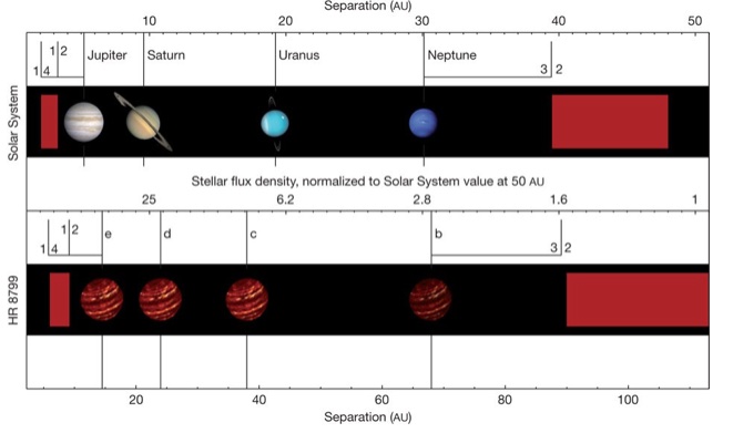
../../_images/hr8799.jpg — Fig. 2.8 The four gas giants and two planetesimal belts orbiting HR 8799 compared to the Solar System’s giant planets, asteroid and Kuiper belt (Marois et al, 2010).#

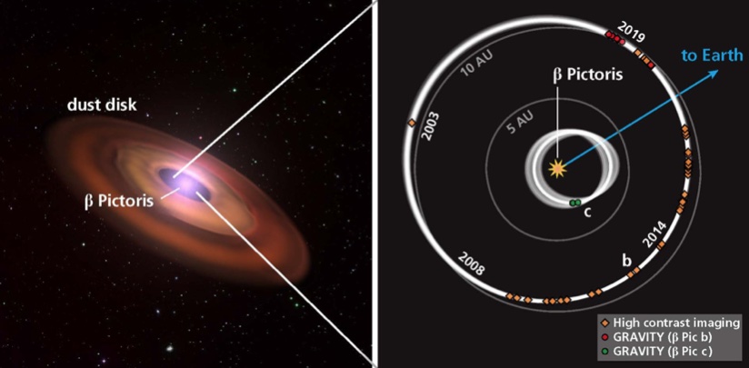
../../_images/betapic.jpg — Fig. 2.9 The \(\beta\) Pic planetary system contains two planets \(\beta\) Pic b orbiting at 10au, with a mass of 11.7\(M_J\) and \(\beta\) Pic c orbiting at 2.68au, with a mass of 10.14\(M_J\) and two dust belts, an inner belt at 6au and an outer belt centred around 90au (Dent et al, 2014, Lagrange et al, 2020).#

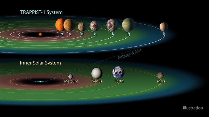
../../_images/trappist_ab.jpeg — Fig. 2.10 The Trappist-1 planetary system orbits a star of mass \(0.08M_\odot\) and contains seven planets within 0.1au (Gillon et al, 2016).#

Limitations on our observational characterisation of Exoplanetary System Architectures#

The key take-away from this lecture is an undersatnding of how our perspective on exoplanetary system architectures is skewed by our ability to detect planets and planetesimal belts. Whilst hot Jupiters dominated the first exoplanet detections, we now know that these systems are quite unusual, they were just the easiest to find. Techniques such as astrometry, showcased by the Gaia space mission, are better suited to detecting planets on longer period orbits, nonetheless our knowledge of architectures beyond a few au remains sparse. The ability to find an Earth on a 1au orbit around a sun-like star, remains the goal of future telescopes, such as the space mission PLAnetary Transits and Oscillations of stars (PLATO) using transits and the Terra-Hunting Experiment, using radial velocity measurements from the ground.

The Radius Valley#

The Kepler space mission revolutionised our understanding of the distribution of exoplanets, enabling population-level statistics. One of the key outcomes from this mission, was the discovery that the distribution of exoplanet radii, unveiled by planetary transits, is bimodal, as shown on Fig. 2.11. There are two peaks, one corresponding to sub-Neptunes of around 2-3 \(R_\oplus\) and the other to super-Earths of around 1.3\(R_\oplus\). Subsequent observations have verified the existence of this radius valley and detailed its exact location and how this varies with additional properties such as stellar mass.

There are several theories that have been put forward to explain the existance of this gap in planetary radii. It is most readily explained by two populations of planets: rocky cores and rocky cores plus gaseous envelopes. If all planets form with large gaseous envelopes, but some planets are stripped of their atmospheres by extreme ultraviolet radiation from the star, the stripped planets become the rocky cores. This theory of photoevaporation is a key contender for explaining the radius valley (Owen & Wu, 2013). Alternatively, as the cores of planets cool and radiate their internal energy to space, this radiation may erode any planetary atmosphere. This theory is known as core-powered mass loss (e.g. Gupta et la, 2019). Particularly for low mass stars, there may be three populations of planets: rocky cores, water-rich and gas-rich planets, with rocky cores forming within the ice-line, whilst water wordls form beyond and migrate inwards (Luque et al, 2022).

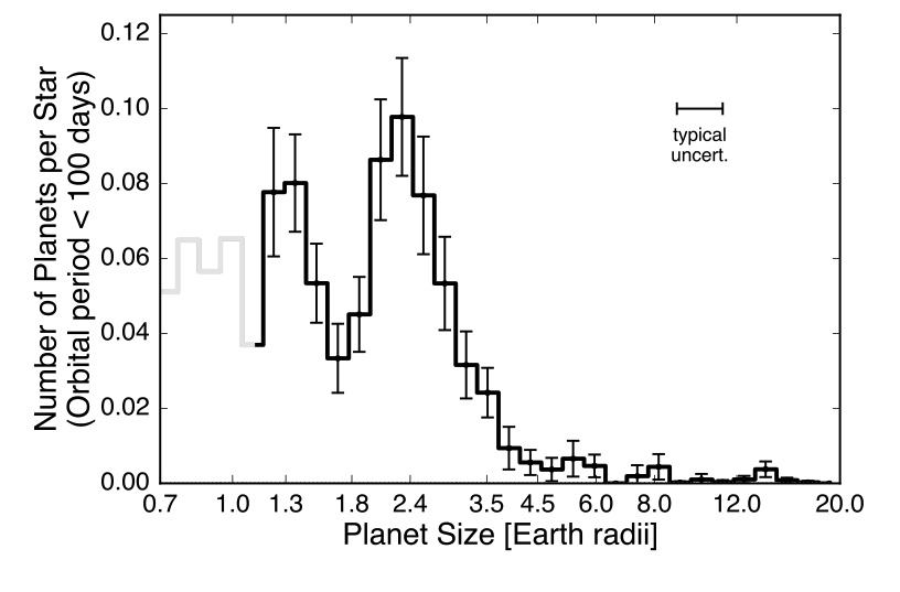
../../_images/fulton.jpg — Fig. 2.11 The completeness-corrected histogram of planet radii for planets with orbital periods shorter than 100days from the California-Kepler Survey (Fulton et al, 2017). The bimodal distribution is known as the mass-radius valley.#

The Habitable Zone#

A key feature of exoplanetary system architectures is whether any planets orbit in the Habitable zone. Astronomers use this to assess the best potential candidates for planets similar to Earth that might be able to host life. The habitable zone is defined as the distance from the star in which liquid water could exist on the planet’s surface. Liquid water being crucial to life on Earth is commonly cited as essential for life beyond Earth.

In the most basic example, the planet intercepts a certain fraction of the star’s irradiation at its orbital distance. The planet remits as a black-body, with an equilibrium temperature of \(T_{\rm eq}\). The emitted flux from the planet of radius \(r\) is given by:

\(F_{\rm emit} = \sigma_{SB} T_{\rm eq}^4 \, 4 \pi r^2 \),

where \(\sigma_{SB}\) is the Stefan-Boltzmann constant. The \(4\pi r^2\) is a result of emission over the full surface area of a sphere. We can equate the emitted flux to the absorbed flux from the star, \(F_*\), taking into account the planet’s albedo, \(A\):

\( (1-A) F_* \pi r^2 = \sigma_{SB} T_{\rm eq}^4 \, 4 \pi r^2 \),

noting that the planet only absorbs the stellar flux across the area presented to the star, \(\pi r^2\). The flux \(F_*\) absorbed by planet is the star’s luminosity divided by the area of the sphere at the location of the planet’s orbit, \(4\pi a_{\rm pl}^2\), such that

\(F_* = \frac{L_*}{4 \pi a^2}\).

Thus, the equlibrium temperature of the planet can be approximated as:

\(T_{\rm eq} = \left ( \frac{L_* (1-A) }{16 \pi \sigma_{SB} \, a^2}\right)^{1/4}\). Liquid water exists between \(0^\circ\) and \(100^\circ\). Thus, the habitable zone is closer to the star for the lower luminosity stars where rocky planets are often found (see Fig. 2.12).

A more realistic version of the habitable zone takes into account the ability of the planetary atmosphere to warm the planet, with the inner edge of the habitable zone being the runaway greenhouse limit and the outer edge the maximum greenhouse limit. The maximum greenhouse limit describes where a CO\(_2\) dominated atmosphere has produced the maximum amount of greenhouse warming and further increases in CO\(_2\) only lead to freeze-out. The runaway greenhouse limit occurs when a planet’s atmosphere contains enough green-house gases that it can no longer cool, such as potentially occurred to Venus.

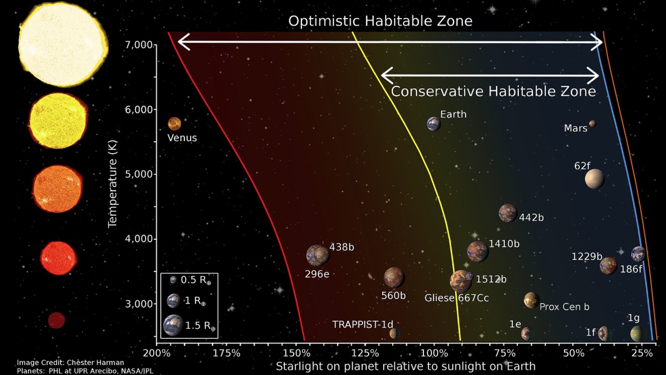
../../_images/hz.jpg — Fig. 2.12 The habitable zone boundary as a function of the starlight received by the planet (relative to Earth) and the star’s temperature (K) Image Credit: Chester Harman.#

Dynamical Stability#

A key feature of exoplanetary systems is their dynamical stability. Dynamical stability is not easy to characterise precisely, with discussion focusing rather on the probability for planet(s) to suffer close encouters within a certain time period. The Solar System’s current planet configuration has been stable for over 5 Gyrs, but there is a non-neglible probability of an instability occurring within the next 5 Gyrs. The eccentricity distribution of observed exoplanets has been linked to dynamical instabilities that occurred in their past (e.g. Carrera et al, 2019).

In general, for a pair of planets, the Hill sphere defines the region around the planet where another body’s trajectory would be domianted by the gravitational influence of the planet, and the gravitational influence of the star or other planets could be neglected. The Hill sphere is given by :

\(R_{H1,2}= \left(\frac{ M_1 + M_2}{3M_*}\right)^{1/3} \frac{a_1+ a_2}{2}\),

where \(a_1\), \(a_2\) are the semi-major axis of the two planets, \(M_1\), \(M_2\), their masses and \(M_*\) the stellar mass.

The stability of a chain of planets can be estimated in terms of their separation in mutual Hill radii:

\(\Delta = \frac{a_2 - a_1}{R_{H1,2}}\)

Chambers et al, 1996 find that planets closer than \(10\Delta\) are always unstable and provide an empirical relationship for the timescale on which planets go unstable, as shown in Fig. 2.13 as a function of mutual Hill radii. Fang & Margot 2013 find that on average neighboring planets in the Kepler exoplanet catalogue are separated by \(21.7R_{H1,2}\). Many exoplanetary systems appear to be dynamically packed, or in other words, additional planets would render the system unstable. This has led to speculation that gaps in many observed exoplanetary systems, including between giant planets or dust belts, may contain additional undetected planets.

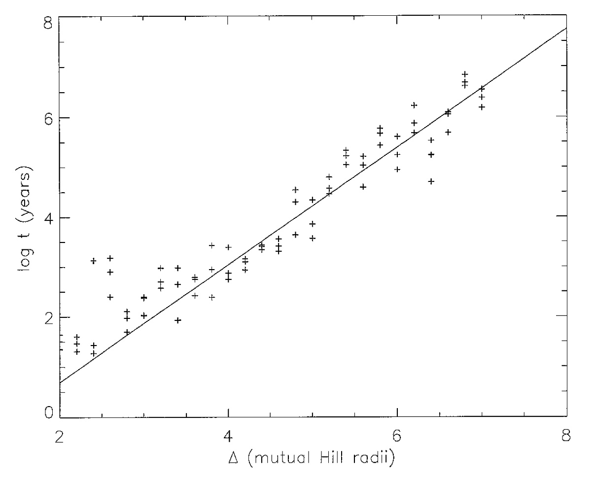
../../_images/chambers.jpg — Fig. 2.13 The timescales (log years) on which three equally spaced \(10^{-7}M_{\odot}\) planets go unstable, when started on intially circular, coplanar orbits (Chambers et al, 1996).#

Resonance Configurations#

Resonance configurations can protect planets against close encouters with one another and thus, render a planetary system stable on longer timescales. A pair of orbits are in orbital resonance if their orbital periods are an exact integer ratio of one another. In the 2:1 orbital resonance, the inner planet orbits twice for every period of the outer planet, as shown in Fig. 2.14. In the 3:2 orbital resonance, the outer planet orbits three times for every two orbits of the inner planet. Many observed exoplanets have periods close to mean-motion or orbital resonances. Resonances can be both stable and unstable, with secular and inclination resonances also playing an important role.

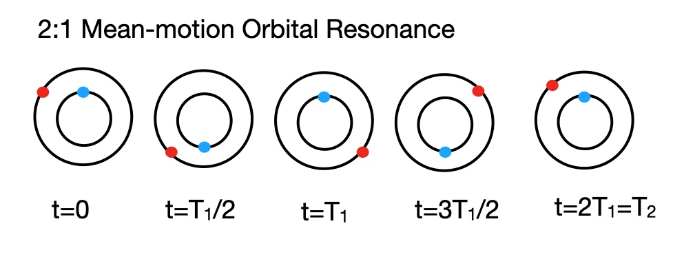
../../_images/resonant21.jpg — Fig. 2.14 A schematic illustrating how two planets (red and blue) in a 2:1 mean-motion orbital resonance would orbit, with time being defined as time in orbital periods of the inner planet, \(T_1\).#

References#

Carrera D., Raymond S.~N., Davies M.~B., 2019, A&A, 629, L7. doi:10.1051/0004-6361/201935744

Chambers J.~E., Wetherill G.~W., Boss A.~P., 1996, Icar, 119, 261. doi:10.1006/icar.19960019

Dent, W. R. F., Wyatt, M. C., Roberge, A., et al. 2014, Sci, 343, 1490

Fang J., Margot J.-L., 2013, ApJ, 767, 115. doi:10.1088/0004-637X/767/2/115

Fulton B.~J., Petigura E.~A., Howard A.~W., Isaacson H., Marcy G.~W., Cargile P.~A., Hebb L., et al., 2017, AJ, 154, 109. doi:10.3847/1538-3881/aa80eb

Gillon M., Jehin E., Lederer S.~M., Delrez L., de Wit J., Burdanov A., Van Grootel V., et al., 2016, Natur, 533, 221. doi:10.1038/nature17448

Gupta A., Schlichting H.~E., 2019, MNRAS, 487, 24. doi:10.1093/mnras/stz1230

Kopparapu et al.(2014), Astrophysical Journal Letters, 787, L29

Lagrange A.~M., Rubini P., Nowak M., Lacour S., Grandjean A., Boccaletti A., Langlois M., et al., 2020, A&A, 642, A18. doi:10.1051/0004-6361/202038823

Luque R., Pall{‘e} E., 2022, Sci, 377, 1211. doi:10.1126/science.abl7164

Marois C., Zuckerman B., Konopacky Q.~M., Macintosh B., Barman T., 2010, Natur, 468, 1080. doi:10.1038/nature09684

Nowak M., Lacour S., Lagrange A.-M., Rubini P., Wang J., Stolker T., Abuter R., et al., 2020, A&A, 642, L2. doi:10.1051/0004-6361/202039039

Owen J.~E., Wu Y., 2013, ApJ, 775, 105. doi:10.1088/0004-637X/775/2/105